++++
++++Notebook converted from Jupyter for blog publishing.
01-PCA-Scikit-Learn
Principal Component Analysis
Imports
import numpy as np
import pandas as pd
import matplotlib.pyplot as plt
import seaborn as sns
Data
Breast cancer wisconsin (diagnostic) dataset
Data Set Characteristics:
:Number of Instances: 569
:Number of Attributes: 30 numeric, predictive attributes and the class
:Attribute Information:
- radius (mean of distances from center to points on the perimeter)
- texture (standard deviation of gray-scale values)
- perimeter
- area
- smoothness (local variation in radius lengths)
- compactness (perimeter^2 / area - 1.0)
- concavity (severity of concave portions of the contour)
- concave points (number of concave portions of the contour)
- symmetry
- fractal dimension ("coastline approximation" - 1)
The mean, standard error, and "worst" or largest (mean of the three worst/largest values) of these features were computed for each image, resulting in 30 features. For instance, field 0 is Mean Radius, field 10 is Radius SE, field 20 is Worst Radius.
- class:
- WDBC-Malignant
- WDBC-Benign
:Summary Statistics:
===================================== ====== ====== Min Max ===================================== ====== ====== radius (mean): 6.981 28.11 texture (mean): 9.71 39.28 perimeter (mean): 43.79 188.5 area (mean): 143.5 2501.0 smoothness (mean): 0.053 0.163 compactness (mean): 0.019 0.345 concavity (mean): 0.0 0.427 concave points (mean): 0.0 0.201 symmetry (mean): 0.106 0.304 fractal dimension (mean): 0.05 0.097 radius (standard error): 0.112 2.873 texture (standard error): 0.36 4.885 perimeter (standard error): 0.757 21.98 area (standard error): 6.802 542.2 smoothness (standard error): 0.002 0.031 compactness (standard error): 0.002 0.135 concavity (standard error): 0.0 0.396 concave points (standard error): 0.0 0.053 symmetry (standard error): 0.008 0.079 fractal dimension (standard error): 0.001 0.03 radius (worst): 7.93 36.04 texture (worst): 12.02 49.54 perimeter (worst): 50.41 251.2 area (worst): 185.2 4254.0 smoothness (worst): 0.071 0.223 compactness (worst): 0.027 1.058 concavity (worst): 0.0 1.252 concave points (worst): 0.0 0.291 symmetry (worst): 0.156 0.664 fractal dimension (worst): 0.055 0.208 ===================================== ====== ======
:Missing Attribute Values: None
:Class Distribution: 212 - Malignant, 357 - Benign
:Creator: Dr. William H. Wolberg, W. Nick Street, Olvi L. Mangasarian
:Donor: Nick Street
:Date: November, 1995
This is a copy of UCI ML Breast Cancer Wisconsin (Diagnostic) datasets. https://goo.gl/U2Uwz2 (opens in a new tab)
Features are computed from a digitized image of a fine needle aspirate (FNA) of a breast mass. They describe characteristics of the cell nuclei present in the image.
Separating plane described above was obtained using Multisurface Method-Tree (MSM-T) [K. P. Bennett, "Decision Tree Construction Via Linear Programming." Proceedings of the 4th Midwest Artificial Intelligence and Cognitive Science Society, pp. 97-101, 1992], a classification method which uses linear programming to construct a decision tree. Relevant features were selected using an exhaustive search in the space of 1-4 features and 1-3 separating planes.
The actual linear program used to obtain the separating plane in the 3-dimensional space is that described in: [K. P. Bennett and O. L. Mangasarian: "Robust Linear Programming Discrimination of Two Linearly Inseparable Sets", Optimization Methods and Software 1, 1992, 23-34].
This database is also available through the UW CS ftp server:
ftp ftp.cs.wisc.edu cd math-prog/cpo-dataset/machine-learn/WDBC/
.. topic:: References
- W.N. Street, W.H. Wolberg and O.L. Mangasarian. Nuclear feature extraction for breast tumor diagnosis. IS&T/SPIE 1993 International Symposium on Electronic Imaging: Science and Technology, volume 1905, pages 861-870, San Jose, CA, 1993.
- O.L. Mangasarian, W.N. Street and W.H. Wolberg. Breast cancer diagnosis and prognosis via linear programming. Operations Research, 43(4), pages 570-577, July-August 1995.
- W.H. Wolberg, W.N. Street, and O.L. Mangasarian. Machine learning techniques to diagnose breast cancer from fine-needle aspirates. Cancer Letters 77 (1994) 163-171.
df = pd.read_csv('../DATA/cancer_tumor_data_features.csv')df.head()mean radius
mean texture
mean perimeter
mean area
mean smoothnessPCA with Scikit-Learn
Scaling Data
from sklearn.preprocessing import StandardScalerscaler = StandardScaler()scaled_X = scaler.fit_transform(df)scaled_Xarray([[ 1.09706398, -2.07333501, 1.26993369, ..., 2.29607613,
2.75062224, 1.93701461],
[ 1.82982061, -0.35363241, 1.68595471, ..., 1.0870843 ,
-0.24388967, 0.28118999],
[ 1.57988811, 0.45618695, 1.56650313, ..., 1.95500035,Scikit-Learn Implementation
from sklearn.decomposition import PCAhelp(PCA)Help on class PCA in module sklearn.decomposition._pca:
class PCA(sklearn.decomposition._base._BasePCA)
| PCA(n_components=None, *, copy=True, whiten=False, svd_solver='auto', tol=0.0, iterated_power='auto', random_state=None)
| pca = PCA(n_components=2)principal_components = pca.fit_transform(scaled_X)plt.figure(figsize=(8,6))
plt.scatter(principal_components[:,0],principal_components[:,1])
plt.xlabel('First principal component')
plt.ylabel('Second Principal Component')Text(0, 0.5, 'Second Principal Component')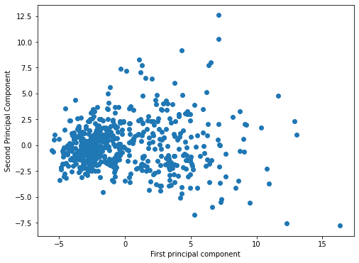
from sklearn.datasets import load_breast_cancer# REQUIRES INTERNET CONNECTION AND FIREWALL ACCESS
cancer_dictionary = load_breast_cancer()cancer_dictionary.keys()dict_keys(['data', 'target', 'frame', 'target_names', 'DESCR', 'feature_names', 'filename'])cancer_dictionary['target']array([0, 0, 0, 0, 0, 0, 0, 0, 0, 0, 0, 0, 0, 0, 0, 0, 0, 0, 0, 1, 1, 1,
0, 0, 0, 0, 0, 0, 0, 0, 0, 0, 0, 0, 0, 0, 0, 1, 0, 0, 0, 0, 0, 0,
0, 0, 1, 0, 1, 1, 1, 1, 1, 0, 0, 1, 0, 0, 1, 1, 1, 1, 0, 1, 0, 0,
1, 1, 1, 1, 0, 1, 0, 0, 1, 0, 1, 0, 0, 1, 1, 1, 0, 0, 1, 0, 0, 0,
1, 1, 1, 0, 1, 1, 0, 0, 1, 1, 1, 0, 0, 1, 1, 1, 1, 0, 1, 1, 0, 1,plt.figure(figsize=(8,6))
plt.scatter(principal_components[:,0],principal_components[:,1],c=cancer_dictionary['target'])
plt.xlabel('First principal component')
plt.ylabel('Second Principal Component')Text(0, 0.5, 'Second Principal Component')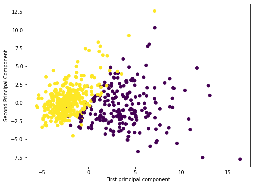
Fitted Model Attributes
pca.n_components2pca.components_array([[ 0.21890244, 0.10372458, 0.22753729, 0.22099499, 0.14258969,
0.23928535, 0.25840048, 0.26085376, 0.13816696, 0.06436335,
0.20597878, 0.01742803, 0.21132592, 0.20286964, 0.01453145,
0.17039345, 0.15358979, 0.1834174 , 0.04249842, 0.10256832,
0.22799663, 0.10446933, 0.23663968, 0.22487053, 0.12795256,In this numpy matrix array, each row represents a principal component, Principal axes in feature space, representing the directions of maximum variance in the data. The components are sorted by explained_variance_.
We can visualize this relationship with a heatmap:
df_comp = pd.DataFrame(pca.components_,index=['PC1','PC2'],columns=df.columns)df_compmean radius
mean texture
mean perimeter
mean area
mean smoothnessplt.figure(figsize=(20,3),dpi=150)
sns.heatmap(df_comp,annot=True)<AxesSubplot:>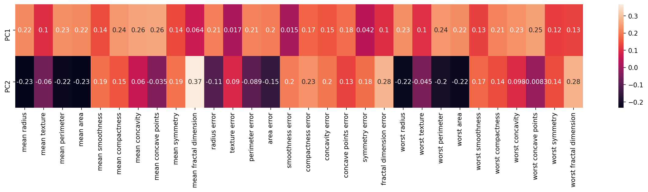
pca.explained_variance_ratio_array([0.44272026, 0.18971182])np.sum(pca.explained_variance_ratio_)0.6324320765155944pca_30 = PCA(n_components=30)
pca_30.fit(scaled_X)PCA(n_components=30)pca_30.explained_variance_ratio_array([4.42720256e-01, 1.89711820e-01, 9.39316326e-02, 6.60213492e-02,
5.49576849e-02, 4.02452204e-02, 2.25073371e-02, 1.58872380e-02,
1.38964937e-02, 1.16897819e-02, 9.79718988e-03, 8.70537901e-03,
8.04524987e-03, 5.23365745e-03, 3.13783217e-03, 2.66209337e-03,
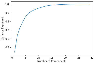
1.97996793e-03, 1.75395945e-03, 1.64925306e-03, 1.03864675e-03,np.sum(pca_30.explained_variance_ratio_)1.0explained_variance = []
for n in range(1,30):
pca = PCA(n_components=n)
pca.fit(scaled_X)
explained_variance.append(np.sum(pca.explained_variance_ratio_))plt.plot(range(1,30),explained_variance)
plt.xlabel("Number of Components")
plt.ylabel("Variance Explained");