++++

Data Science

May 2026×Notebook lesson

Notebook converted from Jupyter for blog publishing.

00-Scatter-Plots

Driptanil DattaSoftware Developer

Scatter Plots

Scatter plots can show how different features are related to one another, the main theme between all relational plot types is they display how features are interconnected to each other. There are many different types of plots that can be used to show this, so let's explore the scatterplot() as well as general seaborn parameters applicable to other plot types.

Data

We'll use some generated data from: http://roycekimmons.com/tools/generated_data (opens in a new tab)

import pandas as pd
import seaborn as sns

df = pd.read_csv("dm_office_sales.csv")

df.head()

division
level of education
training level
work experience
salary

df.info()

<class 'pandas.core.frame.DataFrame'>
RangeIndex: 1000 entries, 0 to 999
Data columns (total 6 columns):
 #   Column              Non-Null Count  Dtype 
---  ------              --------------  ----- 

Scatterplot

sns.scatterplot(x='salary',y='sales',data=df)

<matplotlib.axes._subplots.AxesSubplot at 0x2089e370088>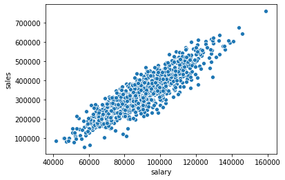

PLOT

Connecting to Figure in Matplotlib

Note how matplotlib is still connected to seaborn underneath (even without importing matplotlib.pyplot), since seaborn itself is directly making a Figure call with matplotlib. We can import matplotlib.pyplot and make calls to directly effect the seaborn figure.

import matplotlib.pyplot as plt

plt.figure(figsize=(12,8))
sns.scatterplot(x='salary',y='sales',data=df)

<matplotlib.axes._subplots.AxesSubplot at 0x2089fb16a08>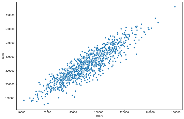

PLOT

Seaborn Parameters

The hue and palette parameters are commonly available around many plot calls in seaborn.

hue

Color points based off a categorical feature in the DataFrame

plt.figure(figsize=(12,8))
sns.scatterplot(x='salary',y='sales',data=df,hue='division')

<matplotlib.axes._subplots.AxesSubplot at 0x2089fb0fe88>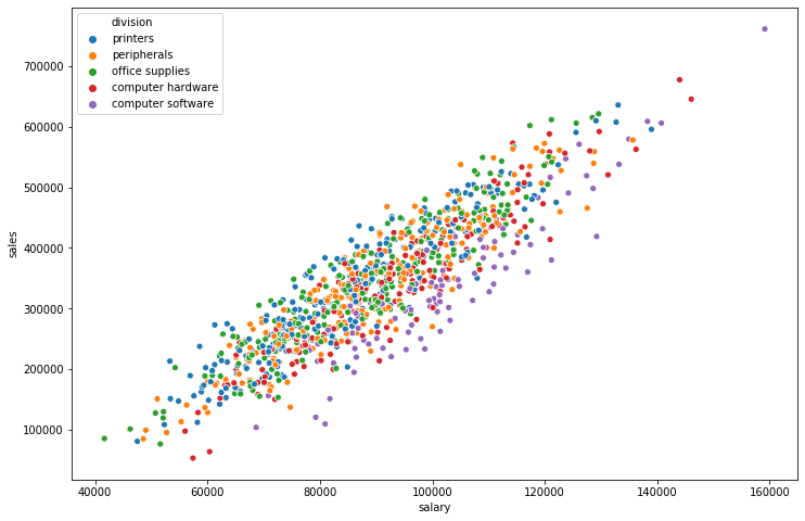

PLOT

plt.figure(figsize=(12,8))
sns.scatterplot(x='salary',y='sales',data=df,hue='work experience')

<matplotlib.axes._subplots.AxesSubplot at 0x2089fc3d848>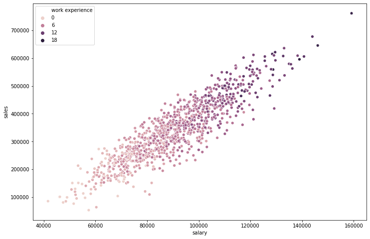

PLOT

Choosing a palette from Matplotlib's cmap: https://matplotlib.org/tutorials/colors/colormaps.html (opens in a new tab)

plt.figure(figsize=(12,8))
sns.scatterplot(x='salary',y='sales',data=df,hue='work experience',palette='viridis')

<matplotlib.axes._subplots.AxesSubplot at 0x2089fcbbdc8>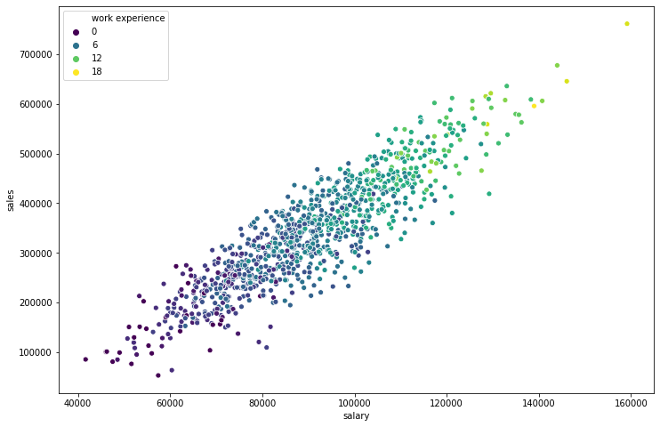

PLOT

Scatterplot Parameters

These parameters are more specific to the scatterplot() call

size

Allows you to size based on another column

plt.figure(figsize=(12,8))
sns.scatterplot(x='salary',y='sales',data=df,size='work experience')

<matplotlib.axes._subplots.AxesSubplot at 0x2089fcb7188>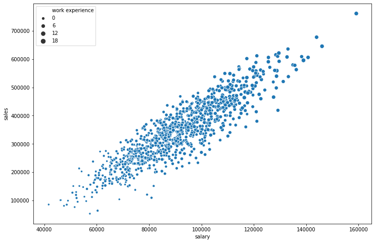

PLOT

Use s= if you want to change the marker size to be some uniform integer value

plt.figure(figsize=(12,8))
sns.scatterplot(x='salary',y='sales',data=df,s=200)

<matplotlib.axes._subplots.AxesSubplot at 0x208a00c1708>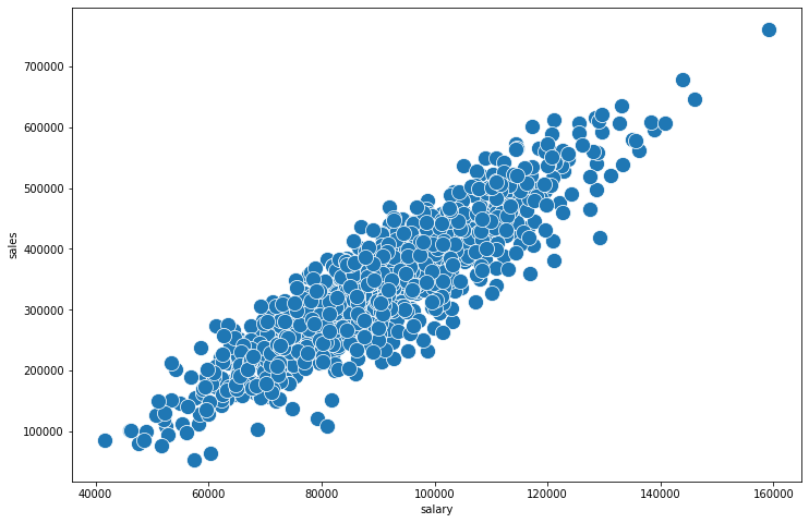

PLOT

plt.figure(figsize=(12,8))
sns.scatterplot(x='salary',y='sales',data=df,s=200,linewidth=0,alpha=0.2)

<matplotlib.axes._subplots.AxesSubplot at 0x208a077b908>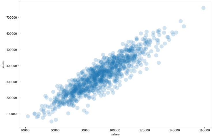

PLOT

style

Automatically choose styles based on another categorical feature in the dataset. Optionally use the markers= parameter to pass a list of marker choices based off matplotlib, for example: ['*','+','o']

plt.figure(figsize=(12,8))
sns.scatterplot(x='salary',y='sales',data=df,style='level of education')

<AxesSubplot:xlabel='salary', ylabel='sales'>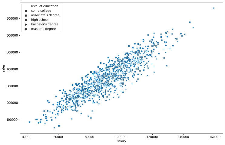

PLOT

plt.figure(figsize=(12,8))
# Sometimes its nice to do BOTH hue and style off the same column
sns.scatterplot(x='salary',y='sales',data=df,style='level of education',hue='level of education',s=100)

<AxesSubplot:xlabel='salary', ylabel='sales'>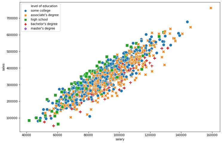

PLOT

Exporting a Seaborn Figure

plt.figure(figsize=(12,8))
sns.scatterplot(x='salary',y='sales',data=df,style='level of education',hue='level of education',s=100)
 
# Call savefig in the same cell
plt.savefig('example_scatter.jpg')

PLOT