++++

Data Science

May 2026×Notebook lesson

Notebook converted from Jupyter for blog publishing.

01-KNN-Exercise

Driptanil DattaSoftware Developer

KNN Project Exercise

Due to the simplicity of KNN for Classification, let's focus on using a PipeLine and a GridSearchCV tool, since these skills can be generalized for any model.

The Sonar Data

Detecting a Rock or a Mine

Sonar (sound navigation ranging) is a technique that uses sound propagation (usually underwater, as in submarine navigation) to navigate, communicate with or detect objects on or under the surface of the water, such as other vessels.

The data set contains the response metrics for 60 separate sonar frequencies sent out against a known mine field (and known rocks). These frequencies are then labeled with the known object they were beaming the sound at (either a rock or a mine).

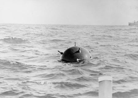
Our main goal is to create a machine learning model capable of detecting the difference between a rock or a mine based on the response of the 60 separate sonar frequencies.

Data Source: https://archive.ics.uci.edu/ml/datasets/Connectionist+Bench+(Sonar,+Mines+vs.+Rocks) (opens in a new tab)

Complete the Tasks in bold

TASK: Run the cells below to load the data.

# !pip install scikit-learn

Requirement already satisfied: scikit-learn in /Users/drippy/.pyenv/versions/3.12.6/lib/python3.12/site-packages (1.7.2)
Requirement already satisfied: numpy>=1.22.0 in /Users/drippy/.pyenv/versions/3.12.6/lib/python3.12/site-packages (from scikit-learn) (2.2.5)
Requirement already satisfied: scipy>=1.8.0 in /Users/drippy/.pyenv/versions/3.12.6/lib/python3.12/site-packages (from scikit-learn) (1.15.2)
Requirement already satisfied: joblib>=1.2.0 in /Users/drippy/.pyenv/versions/3.12.6/lib/python3.12/site-packages (from scikit-learn) (1.5.2)
Requirement already satisfied: threadpoolctl>=3.1.0 in /Users/drippy/.pyenv/versions/3.12.6/lib/python3.12/site-packages (from scikit-learn) (3.6.0)

import numpy as np
import pandas as pd
import seaborn as sns
import matplotlib.pyplot as plt

df = pd.read_csv('../DATA/sonar.all-data.csv')

df.head()

Freq_1
Freq_2
Freq_3
Freq_4
Freq_5

Data Exploration

TASK: Create a heatmap of the correlation between the difference frequency responses.

# CODE HERE
plt.figure(figsize=(8,6))
sns.heatmap(df.select_dtypes(include='number').corr(), cmap='coolwarm')

<Axes: >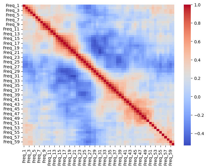

PLOT

TASK: What are the top 5 correlated frequencies with the target\label?

Note: You many need to map the label to 0s and 1s.

Additional Note: We're looking for absolute correlation values.

# create numeric target
df['Target'] = df['Label'].map({'R':0,'M':1})
 
# compute absolute correlations only on numeric columns and show the top 5 features (exclude Target itself)
corrs = df.select_dtypes(include='number').corr()['Target'].abs().sort_values(ascending=True)
top5 = corrs.drop('Target').tail(5)
top5

Freq_45    0.339406
Freq_10    0.341142
Freq_49    0.351312
Freq_12    0.392245
Freq_11    0.432855

Train | Test Split

Our approach here will be one of using Cross Validation on 90% of the dataset, and then judging our results on a final test set of 10% to evaluate our model.

TASK: Split the data into features and labels, and then split into a training set and test set, with 90% for Cross-Validation training, and 10% for a final test set.

Note: The solution uses a random_state=42

from sklearn.model_selection import train_test_split
 
X = df.drop(['Label','Target'], axis=1)
y = df['Target']
 
X_train, X_test, y_train, y_test = train_test_split(X, y, test_size=0.3, random_state=101)

TASK: Create a PipeLine that contains both a StandardScaler and a KNN model

from sklearn.preprocessing import StandardScaler
from sklearn.neighbors import KNeighborsClassifier
from sklearn.pipeline import Pipeline

scalar = StandardScaler()
 
knn = KNeighborsClassifier()

operations = [('scaler', scalar), ('knn', knn)]

pipe = Pipeline(operations)

TASK: Perform a grid-search with the pipeline to test various values of k and report back the best performing parameters.

from sklearn.model_selection import GridSearchCV

k_values = list(range(1,20))
param_grid = {'knn__n_neighbors': k_values}

full_cv_classifier = GridSearchCV(pipe, param_grid, cv=5, scoring='accuracy')
 
full_cv_classifier.fit(X_train, y_train)

GridSearchCV(cv=5,
estimator=Pipeline(steps=[('scaler', StandardScaler()),
('knn', KNeighborsClassifier())]),
param_grid={'knn__n_neighbors': [1, 2, 3, 4, 5, 6, 7, 8, 9, 10, 11,
12, 13, 14, 15, 16, 17, 18, 19]},

(HARD) TASK: Using the .cv_results_ dictionary, see if you can create a plot of the mean test scores per K value.

full_cv_classifier.cv_results_['mean_test_score']

array([0.84137931, 0.84827586, 0.83448276, 0.8       , 0.77241379,
       0.77931034, 0.73103448, 0.74482759, 0.71724138, 0.74482759,
       0.72413793, 0.75862069, 0.71034483, 0.74482759, 0.72413793,
       0.73103448, 0.70344828, 0.70344828, 0.70344828])

plt.figure(figsize=(10,6), dpi=200)
plt.plot(k_values, full_cv_classifier.cv_results_['mean_test_score'], label='Mean Test Score')
plt.legend()
plt.xlabel('K Value')
plt.ylabel('Cross Validated Accuracy')

Text(0, 0.5, 'Cross Validated Accuracy')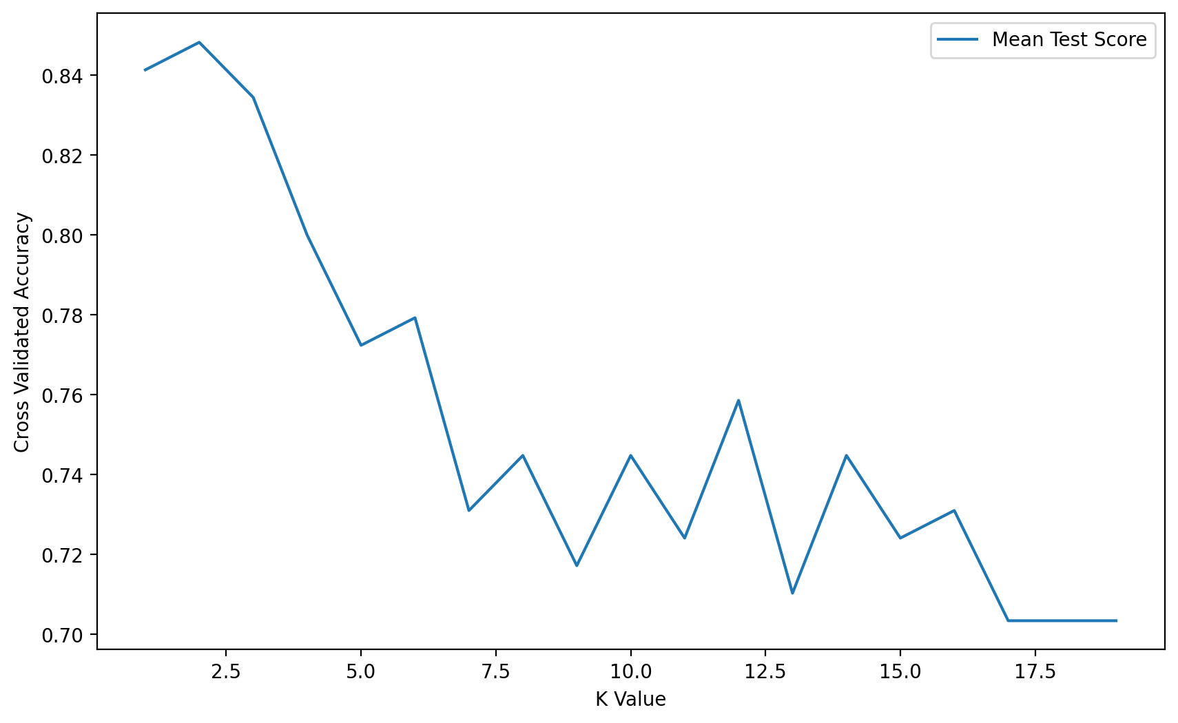

PLOT

Final Model Evaluation

TASK: Using the grid classifier object from the previous step, get a final performance classification report and confusion matrix.

scaler = StandardScaler()
knn8 = KNeighborsClassifier(n_neighbors=8)
operations = [('scaler',scaler),('knn8',knn8)]

pipe = Pipeline(operations)
pipe.fit(X_train,y_train)
pipe_pred = pipe.predict(X_test)

from sklearn.metrics import classification_report
 
print(classification_report(y_test,pipe_pred))

              precision    recall  f1-score   support

           0       0.82      0.70      0.75        33
           1       0.71      0.83      0.77        30

Great Job!