++++

Data Science

May 2026×Notebook lesson

Notebook converted from Jupyter for blog publishing.

01-Capstone-Project-Solutions

Driptanil DattaSoftware Developer

Capstone Project - Solution

Overview

If you are planning on going out to see a movie, how well can you trust online reviews and ratings? Especially if the same company showing the rating also makes money by selling movie tickets. Do they have a bias towards rating movies higher than they should be rated?

Goal:

Your goal is to complete the tasks below based off the 538 article and see if you reach a similar conclusion. You will need to use your pandas and visualization skills to determine if Fandango's ratings in 2015 had a bias towards rating movies better to sell more tickets.

Complete the tasks written in bold.

Part One: Understanding the Background and Data

TASK: Read this article: Be Suspicious Of Online Movie Ratings, Especially Fandango’s (opens in a new tab)

TASK: After reading the article, read these two tables giving an overview of the two .csv files we will be working with:

The Data

This is the data behind the story Be Suspicious Of Online Movie Ratings, Especially Fandango’s (opens in a new tab) openly available on 538's github: https://github.com/fivethirtyeight/data (opens in a new tab). There are two csv files, one with Fandango Stars and Displayed Ratings, and the other with aggregate data for movie ratings from other sites, like Metacritic,IMDB, and Rotten Tomatoes.

all_sites_scores.csv

all_sites_scores.csv{:python} contains every film that has a Rotten Tomatoes rating, a RT User rating, a Metacritic score, a Metacritic User score, and IMDb score, and at least 30 fan reviews on Fandango. The data from Fandango was pulled on Aug. 24, 2015.

Column	Definition
FILM	The film in question
RottenTomatoes	The Rotten Tomatoes Tomatometer score for the film
RottenTomatoes_User	The Rotten Tomatoes user score for the film
Metacritic	The Metacritic critic score for the film
Metacritic_User	The Metacritic user score for the film
IMDB	The IMDb user score for the film
Metacritic_user_vote_count	The number of user votes the film had on Metacritic
IMDB_user_vote_count	The number of user votes the film had on IMDb

fandango_scape.csv

fandango_scrape.csv{:python} contains every film 538 pulled from Fandango.

Column	Definiton
FILM	The movie
STARS	Number of stars presented on Fandango.com
RATING	The Fandango ratingValue for the film, as pulled from the HTML of each page. This is the actual average score the movie obtained.
VOTES	number of people who had reviewed the film at the time we pulled it.

TASK: Import any libraries you think you will use:

# IMPORT HERE!

import numpy as np
import pandas as pd
import matplotlib.pyplot as plt
import seaborn as sns

Part Two: Exploring Fandango Displayed Scores versus True User Ratings

Let's first explore the Fandango ratings to see if our analysis agrees with the article's conclusion.

TASK: Run the cell below to read in the fandango_scrape.csv file

fandango = pd.read_csv("fandango_scrape.csv")

TASK: Explore the DataFrame Properties and Head.

fandango.head()

HTML

FILM
STARS
RATING
VOTES
0

fandango.info()

STDOUT

<class 'pandas.core.frame.DataFrame'>
RangeIndex: 504 entries, 0 to 503
Data columns (total 4 columns):
 #   Column  Non-Null Count  Dtype  
---  ------  --------------  -----

fandango.describe()

HTML

STARS
RATING
VOTES
count
504.000000

TASK: Let's explore the relationship between popularity of a film and its rating. Create a scatterplot showing the relationship between rating and votes. Feel free to edit visual styling to your preference.

# CODE HERE

plt.figure(figsize=(10,4),dpi=150)
sns.scatterplot(data=fandango,x='RATING',y='VOTES');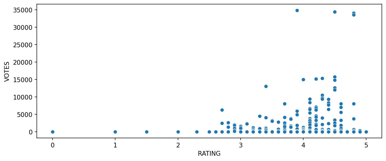

PLOT

TASK: Calculate the correlation between the columns:

# CODE HERE

fandango.corr()

HTML

STARS
RATING
VOTES
STARS
1.000000

TASK: Assuming that every row in the FILM title column has the same format:

Film Title Name (Year)

Create a new column that is able to strip the year from the title strings and set this new column as YEAR

# CODE HERE

fandango['YEAR'] = fandango['FILM'].apply(lambda title:title.split('(')[-1])

TASK: How many movies are in the Fandango DataFrame per year?

#CODE HERE

fandango['YEAR'].value_counts()

RESULT

2015    478
2014     23
2016      1
1964      1
2012      1

TASK: Visualize the count of movies per year with a plot:

#CODE HERE

sns.countplot(data=fandango,x='YEAR')

RESULT

<AxesSubplot:xlabel='YEAR', ylabel='count'>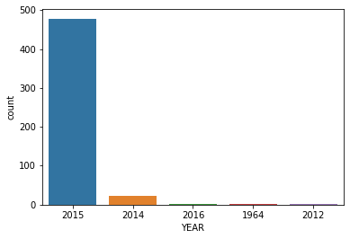

PLOT

TASK: What are the 10 movies with the highest number of votes?

#CODE HERE

fandango.nlargest(10,'VOTES')

HTML

FILM
STARS
RATING
VOTES
YEAR

TASK: How many movies have zero votes?

#CODE HERE

no_votes = fandango['VOTES']==0 
no_votes.sum()

RESULT

TASK: Create DataFrame of only reviewed films by removing any films that have zero votes.

#CODE HERE

fan_reviewed = fandango[fandango['VOTES']>0]

As noted in the article, due to HTML and star rating displays, the true user rating may be slightly different than the rating shown to a user. Let's visualize this difference in distributions.

TASK: Create a KDE plot (or multiple kdeplots) that displays the distribution of ratings that are displayed (STARS) versus what the true rating was from votes (RATING). Clip the KDEs to 0-5.

#CODE HERE

plt.figure(figsize=(10,4),dpi=150)
sns.kdeplot(data=fan_reviewed,x='RATING',clip=[0,5],fill=True,label='True Rating')
sns.kdeplot(data=fan_reviewed,x='STARS',clip=[0,5],fill=True,label='Stars Displayed')
 
plt.legend(loc=(1.05,0.5))

RESULT

<matplotlib.legend.Legend at 0x1aa0110cdc8>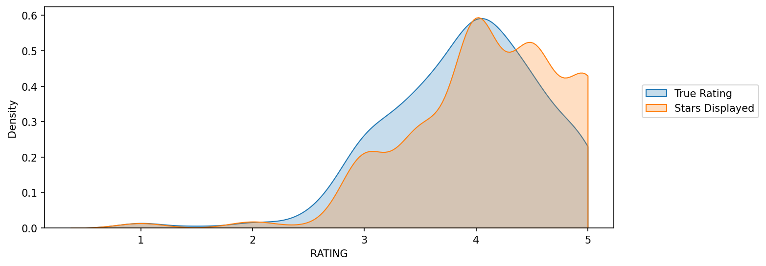

PLOT

TASK: Let's now actually quantify this discrepancy. Create a new column of the different between STARS displayed versus true RATING. Calculate this difference with STARS-RATING and round these differences to the nearest decimal point.

#CODE HERE

fan_reviewed["STARS_DIFF"] = fan_reviewed['STARS'] - fan_reviewed['RATING'] 
fan_reviewed['STARS_DIFF'] = fan_reviewed['STARS_DIFF'].round(2)

fan_reviewed

HTML

FILM
STARS
RATING
VOTES
YEAR

TASK: Create a count plot to display the number of times a certain difference occurs:

#CODE HERE

plt.figure(figsize=(12,4),dpi=150)
sns.countplot(data=fan_reviewed,x='STARS_DIFF',palette='magma')

RESULT

<AxesSubplot:xlabel='STARS_DIFF', ylabel='count'>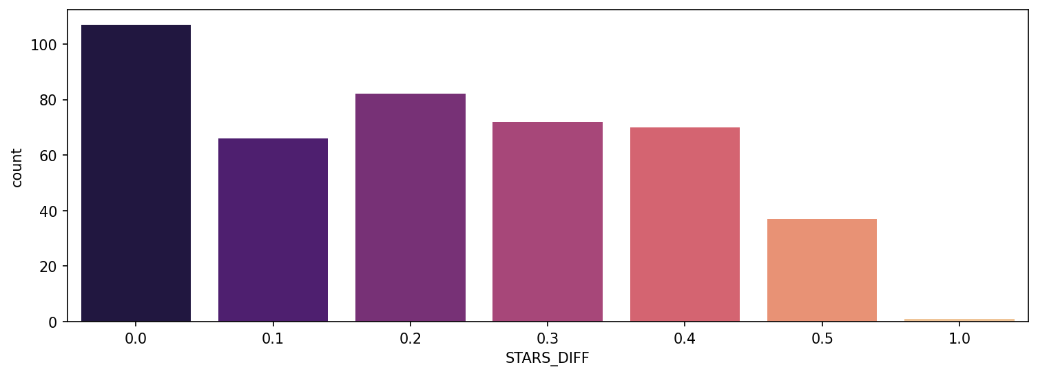

PLOT

TASK: We can see from the plot that one movie was displaying over a 1 star difference than its true rating! What movie had this close to 1 star differential?

#CODE HERE

fan_reviewed[fan_reviewed['STARS_DIFF'] == 1]

HTML

FILM
STARS
RATING
VOTES
YEAR

Part Three: Comparison of Fandango Ratings to Other Sites

Let's now compare the scores from Fandango to other movies sites and see how they compare.

TASK: Read in the "all_sites_scores.csv" file by running the cell below

all_sites = pd.read_csv("all_sites_scores.csv")

TASK: Explore the DataFrame columns, info, description.

all_sites.head()

HTML

FILM
RottenTomatoes
RottenTomatoes_User
Metacritic
Metacritic_User

all_sites.info()

STDOUT

<class 'pandas.core.frame.DataFrame'>
RangeIndex: 146 entries, 0 to 145
Data columns (total 8 columns):
 #   Column                      Non-Null Count  Dtype  
---  ------                      --------------  -----

all_sites.describe()

HTML

RottenTomatoes
RottenTomatoes_User
Metacritic
Metacritic_User
IMDB

Rotten Tomatoes

Let's first take a look at Rotten Tomatoes. RT has two sets of reviews, their critics reviews (ratings published by official critics) and user reviews.

TASK: Create a scatterplot exploring the relationship between RT Critic reviews and RT User reviews.

# CODE HERE

plt.figure(figsize=(10,4),dpi=150)
sns.scatterplot(data=all_sites,x='RottenTomatoes',y='RottenTomatoes_User')
plt.xlim(0,100)
plt.ylim(0,100)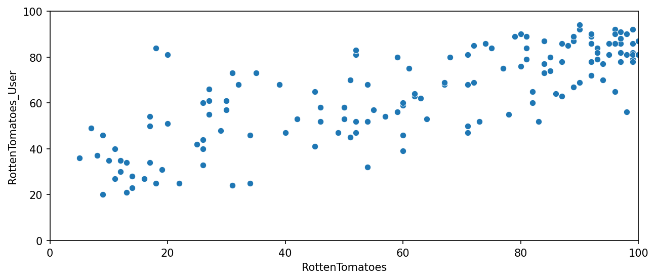

RESULT

(0.0, 100.0)

PLOT

Let's quantify this difference by comparing the critics ratings and the RT User ratings. We will calculate this with RottenTomatoes-RottenTomatoes_User. Note: Rotten_Diff here is Critics - User Score. So values closer to 0 means aggrement between Critics and Users. Larger positive values means critics rated much higher than users. Larger negative values means users rated much higher than critics.

TASK: Create a new column based off the difference between critics ratings and users ratings for Rotten Tomatoes. Calculate this with RottenTomatoes-RottenTomatoes_User

#CODE HERE

all_sites['Rotten_Diff']  = all_sites['RottenTomatoes'] - all_sites['RottenTomatoes_User']

Let's now compare the overall mean difference. Since we're dealing with differences that could be negative or positive, first take the absolute value of all the differences, then take the mean. This would report back on average to absolute difference between the critics rating versus the user rating.

TASK: Calculate the Mean Absolute Difference between RT scores and RT User scores as described above.

# CODE HERE

all_sites['Rotten_Diff'].apply(abs).mean()

RESULT

15.095890410958905

TASK: Plot the distribution of the differences between RT Critics Score and RT User Score. There should be negative values in this distribution plot. Feel free to use KDE or Histograms to display this distribution.

#CODE HERE

plt.figure(figsize=(10,4),dpi=200)
sns.histplot(data=all_sites,x='Rotten_Diff',kde=True,bins=25)
plt.title("RT Critics Score minus RT User Score");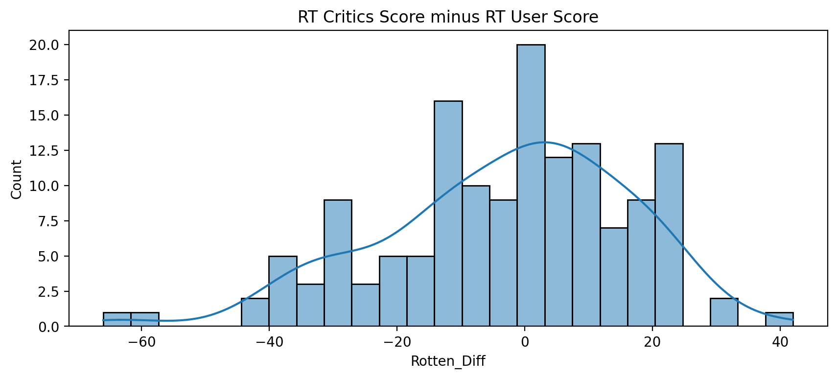

PLOT

TASK: Now create a distribution showing the absolute value difference between Critics and Users on Rotten Tomatoes.

#CODE HERE

plt.figure(figsize=(10,4),dpi=200)
sns.histplot(x=all_sites['Rotten_Diff'].apply(abs),bins=25,kde=True)
plt.title("Abs Difference between RT Critics Score and RT User Score");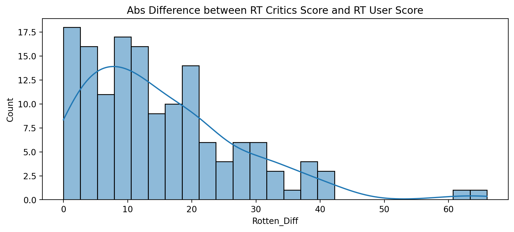

PLOT

Let's find out which movies are causing the largest differences. First, show the top 5 movies with the largest negative difference between Users and RT critics. Since we calculated the difference as Critics Rating - Users Rating, then large negative values imply the users rated the movie much higher on average than the critics did.

TASK: What are the top 5 movies users rated higher than critics on average:

# CODE HERE

print("Users Love but Critics Hate")
all_sites.nsmallest(5,'Rotten_Diff')[['FILM','Rotten_Diff']]

STDOUT

Users Love but Critics Hate

HTML

FILM
Rotten_Diff
3
Do You Believe? (2015)
-66

TASK: Now show the top 5 movies critics scores higher than users on average.

# CODE HERE

print("Critics love, but Users Hate")
all_sites.nlargest(5,'Rotten_Diff')[['FILM','Rotten_Diff']]

STDOUT

Critics love, but Users Hate

HTML

FILM
Rotten_Diff
69
Mr. Turner (2014)
42

MetaCritic

Now let's take a quick look at the ratings from MetaCritic. Metacritic also shows an average user rating versus their official displayed rating.

TASK: Display a scatterplot of the Metacritic Rating versus the Metacritic User rating.

# CODE HERE

plt.figure(figsize=(10,4),dpi=150)
sns.scatterplot(data=all_sites,x='Metacritic',y='Metacritic_User')
plt.xlim(0,100)
plt.ylim(0,10)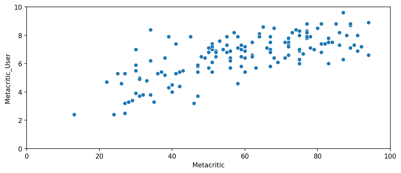

RESULT

(0.0, 10.0)

PLOT

IMBD

Finally let's explore IMDB. Notice that both Metacritic and IMDB report back vote counts. Let's analyze the most popular movies.

TASK: Create a scatterplot for the relationship between vote counts on MetaCritic versus vote counts on IMDB.

#CODE HERE

plt.figure(figsize=(10,4),dpi=150)
sns.scatterplot(data=all_sites,x='Metacritic_user_vote_count',y='IMDB_user_vote_count')

RESULT

<AxesSubplot:xlabel='Metacritic_user_vote_count', ylabel='IMDB_user_vote_count'>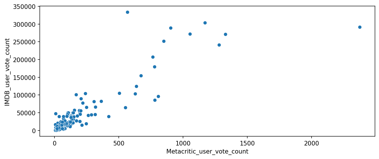

PLOT

Notice there are two outliers here. The movie with the highest vote count on IMDB only has about 500 Metacritic ratings. What is this movie?

TASK: What movie has the highest IMDB user vote count?

#CODE HERE

all_sites.nlargest(1,'IMDB_user_vote_count')

HTML

FILM
RottenTomatoes
RottenTomatoes_User
Metacritic
Metacritic_User

TASK: What movie has the highest Metacritic User Vote count?

#CODE HERE

all_sites.nlargest(1,'Metacritic_user_vote_count')

HTML

FILM
RottenTomatoes
RottenTomatoes_User
Metacritic
Metacritic_User

Fandago Scores vs. All Sites

Finally let's begin to explore whether or not Fandango artificially displays higher ratings than warranted to boost ticket sales.

TASK: Combine the Fandango Table with the All Sites table. Not every movie in the Fandango table is in the All Sites table, since some Fandango movies have very little or no reviews. We only want to compare movies that are in both DataFrames, so do an inner merge to merge together both DataFrames based on the FILM columns.

#CODE HERE

df = pd.merge(fandango,all_sites,on='FILM',how='inner')

df.info()

STDOUT

<class 'pandas.core.frame.DataFrame'>
Int64Index: 145 entries, 0 to 144
Data columns (total 13 columns):
 #   Column                      Non-Null Count  Dtype  
---  ------                      --------------  -----

df.head()

HTML

FILM
STARS
RATING
VOTES
YEAR

Normalize columns to Fandango STARS and RATINGS 0-5

Notice that RT,Metacritic, and IMDB don't use a score between 0-5 stars like Fandango does. In order to do a fair comparison, we need to normalize these values so they all fall between 0-5 stars and the relationship between reviews stays the same.

TASK: Create new normalized columns for all ratings so they match up within the 0-5 star range shown on Fandango. There are many ways to do this.

Hint link: https://stackoverflow.com/questions/26414913/normalize-columns-of-pandas-data-frame (opens in a new tab)

Easier Hint:

Keep in mind, a simple way to convert ratings:

100/20 = 5
10/2 = 5

# CODE HERE

# Dont run this cell multiple times, otherwise you keep dividing!
df['RT_Norm'] = np.round(df['RottenTomatoes']/20,1)
df['RTU_Norm'] =  np.round(df['RottenTomatoes_User']/20,1)

# Dont run this cell multiple times, otherwise you keep dividing!
df['Meta_Norm'] =  np.round(df['Metacritic']/20,1)
df['Meta_U_Norm'] =  np.round(df['Metacritic_User']/2,1)

# Dont run this cell multiple times, otherwise you keep dividing!
df['IMDB_Norm'] = np.round(df['IMDB']/2,1)

df.head()

HTML

FILM
STARS
RATING
VOTES
YEAR

TASK: Now create a norm_scores DataFrame that only contains the normalizes ratings. Include both STARS and RATING from the original Fandango table.

#CODE HERE

norm_scores = df[['STARS','RATING','RT_Norm','RTU_Norm','Meta_Norm','Meta_U_Norm','IMDB_Norm']]

norm_scores.head()

HTML

STARS
RATING
RT_Norm
RTU_Norm
Meta_Norm

Comparing Distribution of Scores Across Sites

Now the moment of truth! Does Fandango display abnormally high ratings? We already know it pushs displayed RATING higher than STARS, but are the ratings themselves higher than average?

TASK: Create a plot comparing the distributions of normalized ratings across all sites. There are many ways to do this, but explore the Seaborn KDEplot docs for some simple ways to quickly show this. Don't worry if your plot format does not look exactly the same as ours, as long as the differences in distribution are clear.

Quick Note if you have issues moving the legend for a seaborn kdeplot: https://github.com/mwaskom/seaborn/issues/2280 (opens in a new tab)

#CODE HERE

def move_legend(ax, new_loc, **kws):
    old_legend = ax.legend_
    handles = old_legend.legendHandles
    labels = [t.get_text() for t in old_legend.get_texts()]
    title = old_legend.get_title().get_text()
    ax.legend(handles, labels, loc=new_loc, title=title, **kws)

fig, ax = plt.subplots(figsize=(15,6),dpi=150)
sns.kdeplot(data=norm_scores,clip=[0,5],shade=True,palette='Set1',ax=ax)
move_legend(ax, "upper left")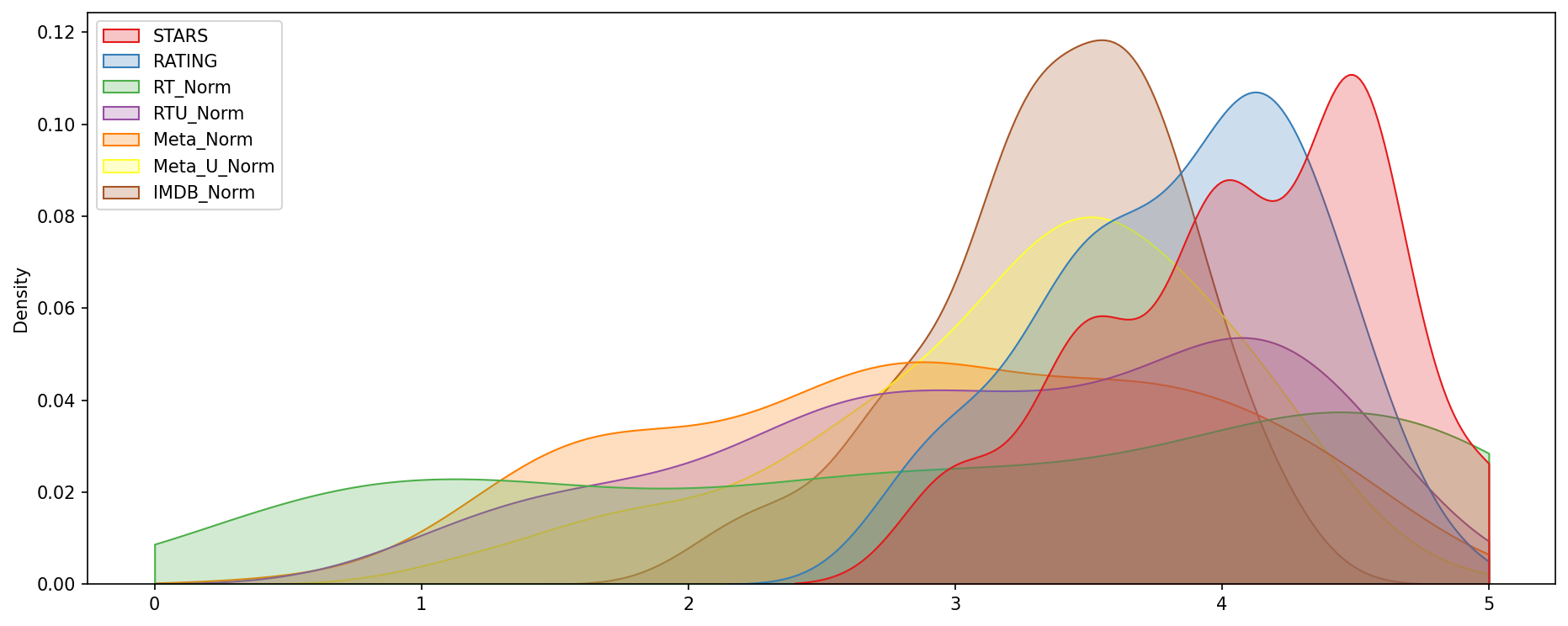

PLOT

Clearly Fandango has an uneven distribution. We can also see that RT critics have the most uniform distribution. Let's directly compare these two.

TASK: Create a KDE plot that compare the distribution of RT critic ratings against the STARS displayed by Fandango.

#CODE HERE

fig, ax = plt.subplots(figsize=(15,6),dpi=150)
sns.kdeplot(data=norm_scores[['RT_Norm','STARS']],clip=[0,5],shade=True,palette='Set1',ax=ax)
move_legend(ax, "upper left")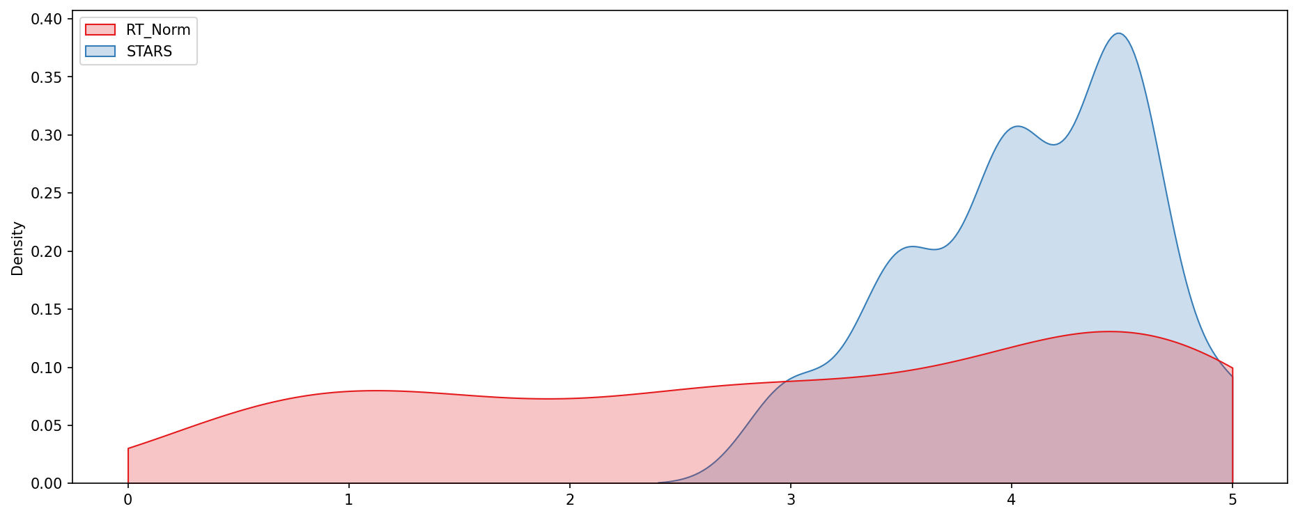

PLOT

OPTIONAL TASK: Create a histplot comparing all normalized scores.

#CODE HERE

plt.subplots(figsize=(15,6),dpi=150)
sns.histplot(norm_scores,bins=50)

RESULT

<AxesSubplot:ylabel='Count'>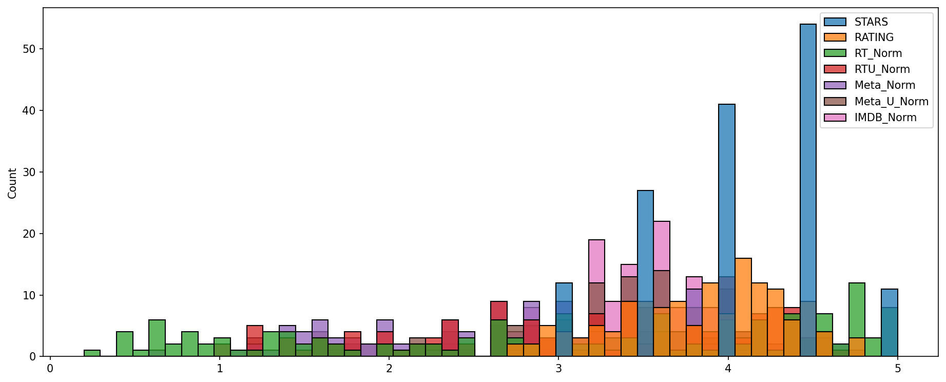

PLOT

How are the worst movies rated across all platforms?

TASK: Create a clustermap visualization of all normalized scores. Note the differences in ratings, highly rated movies should be clustered together versus poorly rated movies. Note: This clustermap does not need to have the FILM titles as the index, feel free to drop it for the clustermap.

# CODE HERE

sns.clustermap(norm_scores,cmap='magma',col_cluster=False)

RESULT

<seaborn.matrix.ClusterGrid at 0x1aa7cb2b548>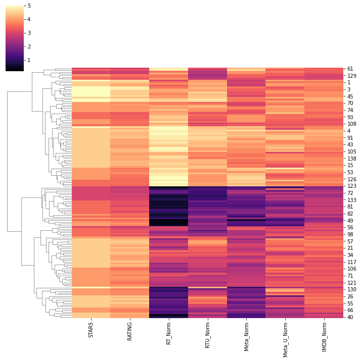

PLOT

TASK: Clearly Fandango is rating movies much higher than other sites, especially considering that it is then displaying a rounded up version of the rating. Let's examine the top 10 worst movies. Based off the Rotten Tomatoes Critic Ratings, what are the top 10 lowest rated movies? What are the normalized scores across all platforms for these movies? You may need to add the FILM column back in to your DataFrame of normalized scores to see the results.

# CODE HERE

norm_films = df[['STARS','RATING','RT_Norm','RTU_Norm','Meta_Norm','Meta_U_Norm','IMDB_Norm','FILM']]

norm_films.nsmallest(10,'RT_Norm')

HTML

STARS
RATING
RT_Norm
RTU_Norm
Meta_Norm

FINAL TASK: Visualize the distribution of ratings across all sites for the top 10 worst movies.

# CODE HERE

print('\n\n')
plt.figure(figsize=(15,6),dpi=150)
worst_films = norm_films.nsmallest(10,'RT_Norm').drop('FILM',axis=1)
sns.kdeplot(data=worst_films,clip=[0,5],shade=True,palette='Set1')
plt.title("Ratings for RT Critic's 10 Worst Reviewed Films");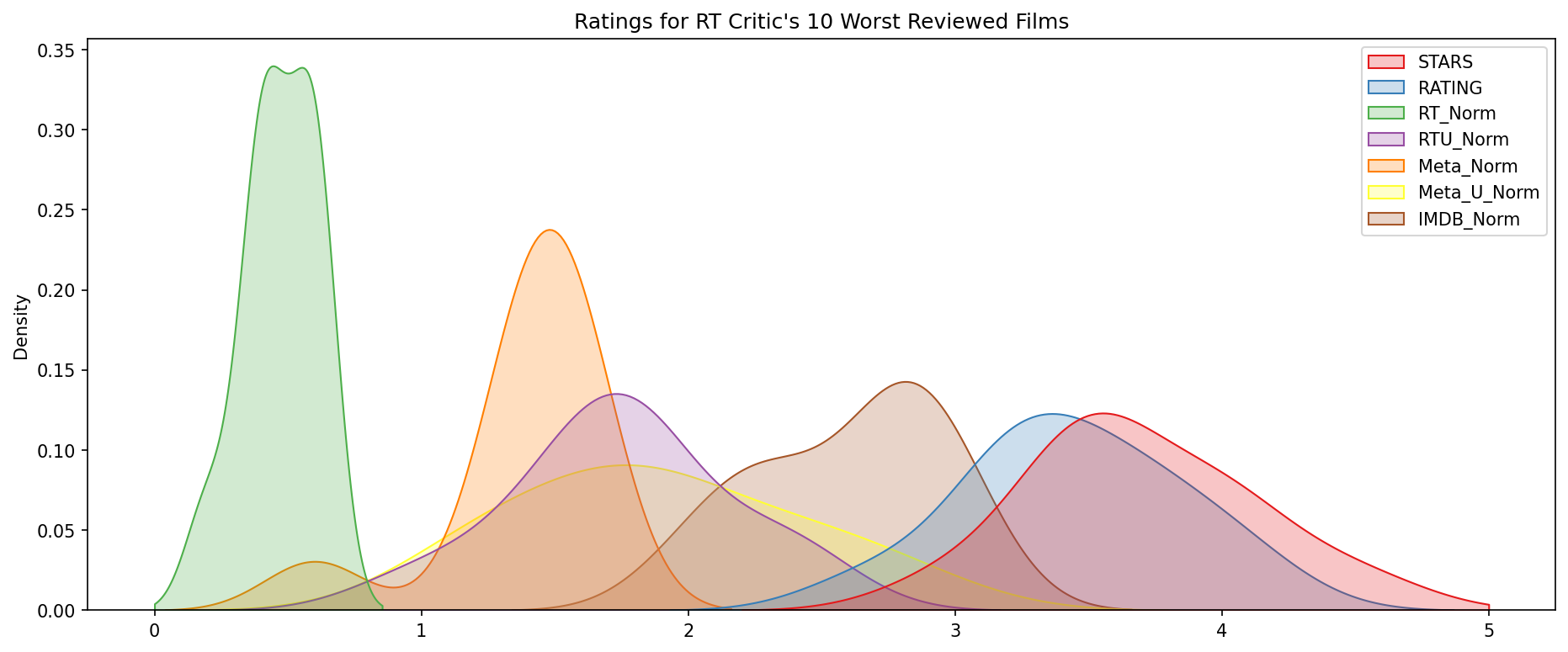

PLOT

Final thoughts: Wow! Fandango is showing around 3-4 star ratings for films that are clearly bad! Notice the biggest offender, Taken 3! (opens in a new tab). Fandango is displaying 4.5 stars on their site for a film with an average rating of 1.86 (opens in a new tab) across the other platforms!

norm_films.iloc[25]

RESULT

STARS                     4.5
RATING                    4.1
RT_Norm                   0.4
RTU_Norm                  2.3
Meta_Norm                 1.3

0.4+2.3+1.3+2.3+3

RESULT

9.3

9.3/5

RESULT

1.86

00 Capstone Project Capstone Project