++++

Data Science

May 2026×Notebook lesson

Notebook converted from Jupyter for blog publishing.

00-Kmeans-Clustering

Driptanil DattaSoftware Developer

K-Means Clustering

Let's work through an example of unsupervised learning - clustering customer data.

Goal:

When working with unsupervised learning methods, its usually important to lay out a general goal. In our case, let's attempt to find reasonable clusters of customers for marketing segmentation and study. What we end up doing with those clusters would depend heavily on the domain itself, in this case, marketing.

The Data

LINK: https://archive.ics.uci.edu/ml/datasets/bank+marketing (opens in a new tab)

This dataset is public available for research. The details are described in [Moro et al., 2011].

[Moro et al., 2011] S. Moro, R. Laureano and P. Cortez. Using Data Mining for Bank Direct Marketing: An Application of the CRISP-DM Methodology. In P. Novais et al. (Eds.), Proceedings of the European Simulation and Modelling Conference - ESM'2011, pp. 117-121, Guimarães, Portugal, October, 2011. EUROSIS.

Available at: [pdf] http://hdl.handle.net/1822/14838 (opens in a new tab) [bib] http://www3.dsi.uminho.pt/pcortez/bib/2011-esm-1.txt (opens in a new tab) For more information, read [Moro et al., 2011].

bank client data:

1 - age (numeric) 2 - job : type of job (categorical: 'admin.','blue-collar','entrepreneur','housemaid','management','retired','self-employed','services','student','technician','unemployed','unknown') 3 - marital : marital status (categorical: 'divorced','married','single','unknown'; note: 'divorced' means divorced or widowed) 4 - education (categorical: 'basic.4y','basic.6y','basic.9y','high.school','illiterate','professional.course','university.degree','unknown') 5 - default: has credit in default? (categorical: 'no','yes','unknown') 6 - housing: has housing loan? (categorical: 'no','yes','unknown') 7 - loan: has personal loan? (categorical: 'no','yes','unknown')

related with the last contact of the current campaign:

8 - contact: contact communication type (categorical: 'cellular','telephone') 9 - month: last contact month of year (categorical: 'jan', 'feb', 'mar', ..., 'nov', 'dec') 10 - day_of_week: last contact day of the week (categorical: 'mon','tue','wed','thu','fri') 11 - duration: last contact duration, in seconds (numeric). Important note: this attribute highly affects the output target (e.g., if duration=0 then y='no'). Yet, the duration is not known before a call is performed. Also, after the end of the call y is obviously known. Thus, this input should only be included for benchmark purposes and should be discarded if the intention is to have a realistic predictive model.

other attributes:

12 - campaign: number of contacts performed during this campaign and for this client (numeric, includes last contact) 13 - pdays: number of days that passed by after the client was last contacted from a previous campaign (numeric; 999 means client was not previously contacted) 14 - previous: number of contacts performed before this campaign and for this client (numeric) 15 - poutcome: outcome of the previous marketing campaign (categorical: 'failure','nonexistent','success')

social and economic context attributes

16 - emp.var.rate: employment variation rate - quarterly indicator (numeric) 17 - cons.price.idx: consumer price index - monthly indicator (numeric) 18 - cons.conf.idx: consumer confidence index - monthly indicator (numeric) 19 - euribor3m: euribor 3 month rate - daily indicator (numeric) 20 - nr.employed: number of employees - quarterly indicator (numeric) 21 - y - has the client subscribed a term deposit? (binary: 'yes','no')

Imports

import numpy as np
import pandas as pd
import matplotlib.pyplot as plt
import seaborn as sns

Exploratory Data Analysis

df = pd.read_csv("../DATA/bank-full.csv")

df.head()

age
job
marital
education
default

df.columns

Index(['age', 'job', 'marital', 'education', 'default', 'housing', 'loan',
       'contact', 'month', 'day_of_week', 'duration', 'campaign', 'pdays',
       'previous', 'poutcome', 'emp.var.rate', 'cons.price.idx',
       'cons.conf.idx', 'euribor3m', 'nr.employed', 'subscribed'],
      dtype='object')

df.info()

<class 'pandas.core.frame.DataFrame'>
RangeIndex: 41188 entries, 0 to 41187
Data columns (total 21 columns):
 #   Column          Non-Null Count  Dtype  
---  ------          --------------  -----  

Continuous Feature Analysis

plt.figure(figsize=(12,6),dpi=200)
sns.histplot(data=df,x='age')

<AxesSubplot:xlabel='age', ylabel='Count'>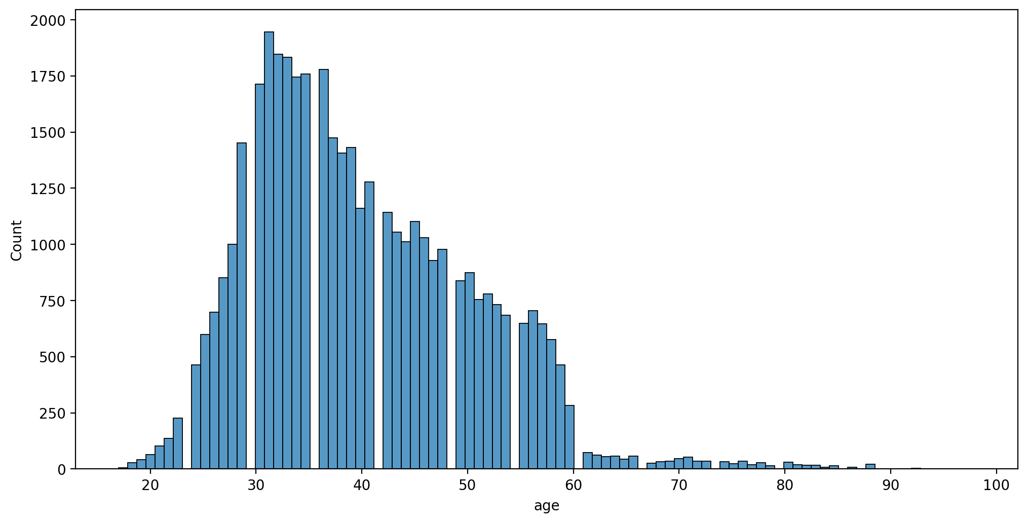

PLOT

plt.figure(figsize=(12,6),dpi=200)
sns.histplot(data=df,x='age',hue='loan')

<AxesSubplot:xlabel='age', ylabel='Count'>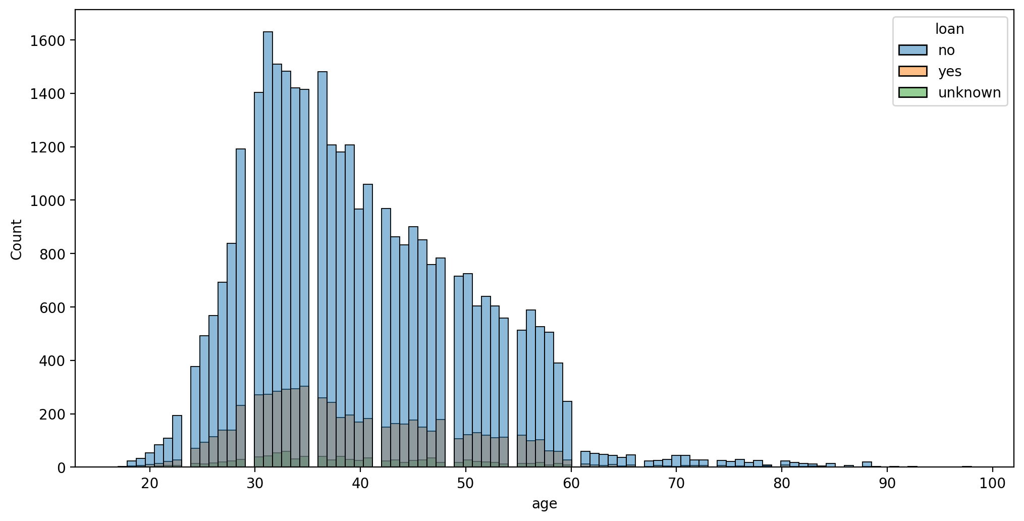

PLOT

plt.figure(figsize=(12,6),dpi=200)
sns.histplot(data=df,x='pdays')

<AxesSubplot:xlabel='pdays', ylabel='Count'>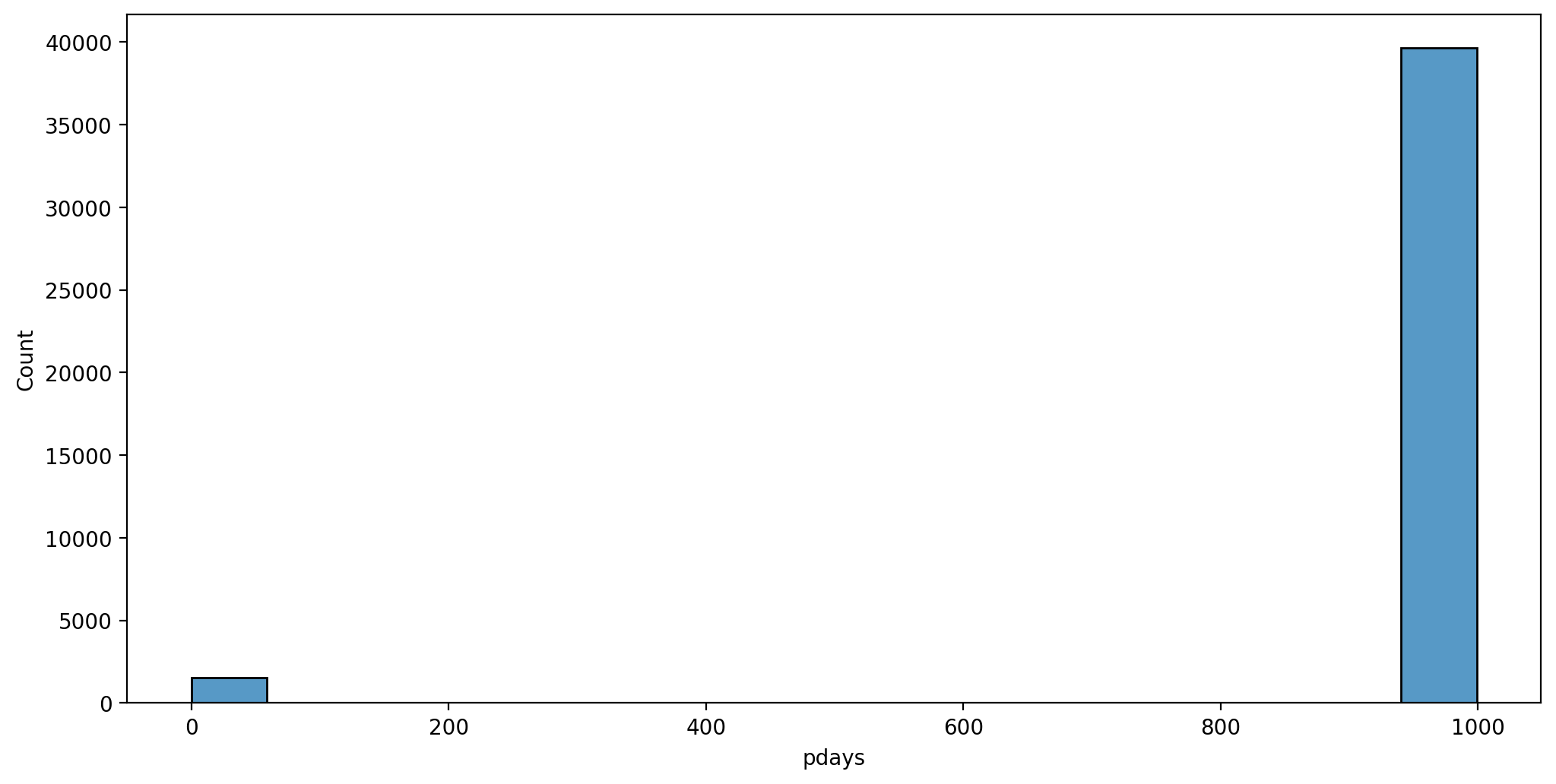

PLOT

plt.figure(figsize=(12,6),dpi=200)
sns.histplot(data=df[df['pdays']!=999],x='pdays')

<AxesSubplot:xlabel='pdays', ylabel='Count'>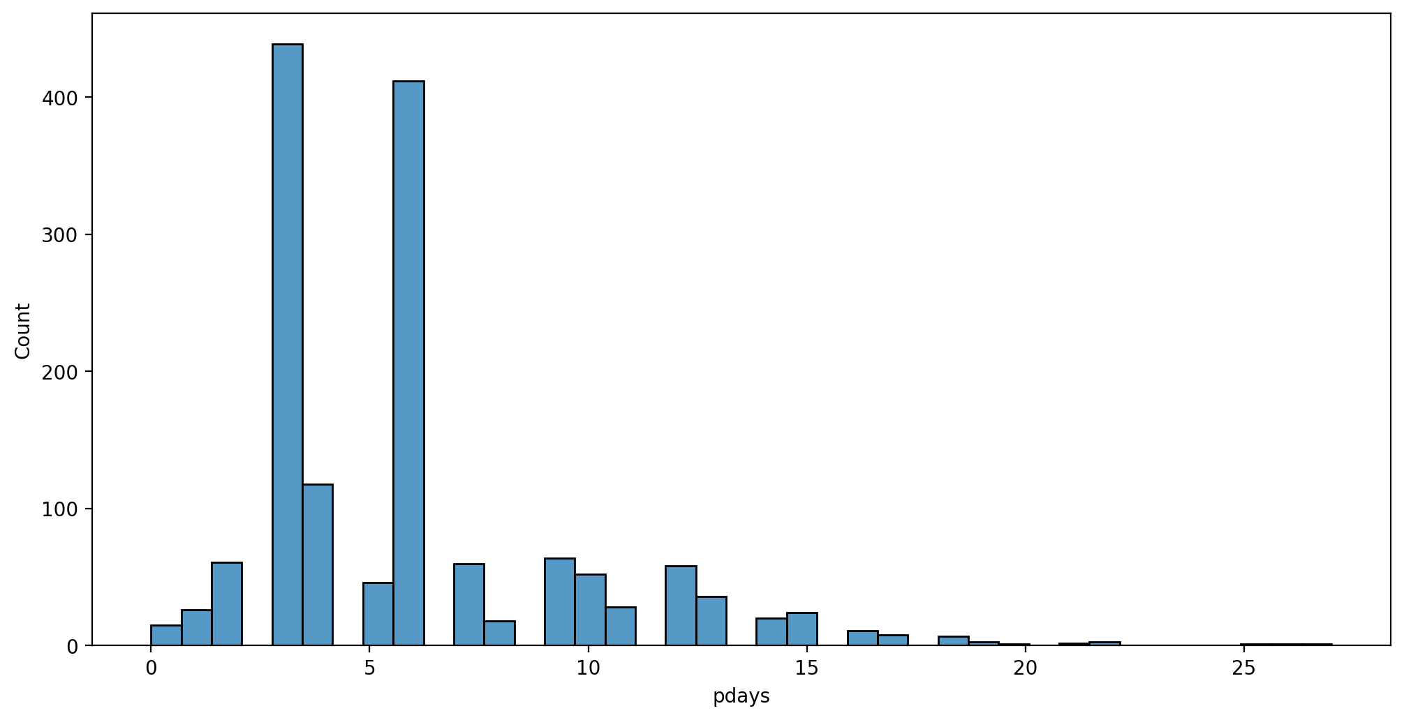

PLOT

Contact duration - contact with customer made, how long did call last?

plt.figure(figsize=(12,6),dpi=200)
sns.histplot(data=df,x='duration',hue='contact')
plt.xlim(0,2000)

(0.0, 2000.0)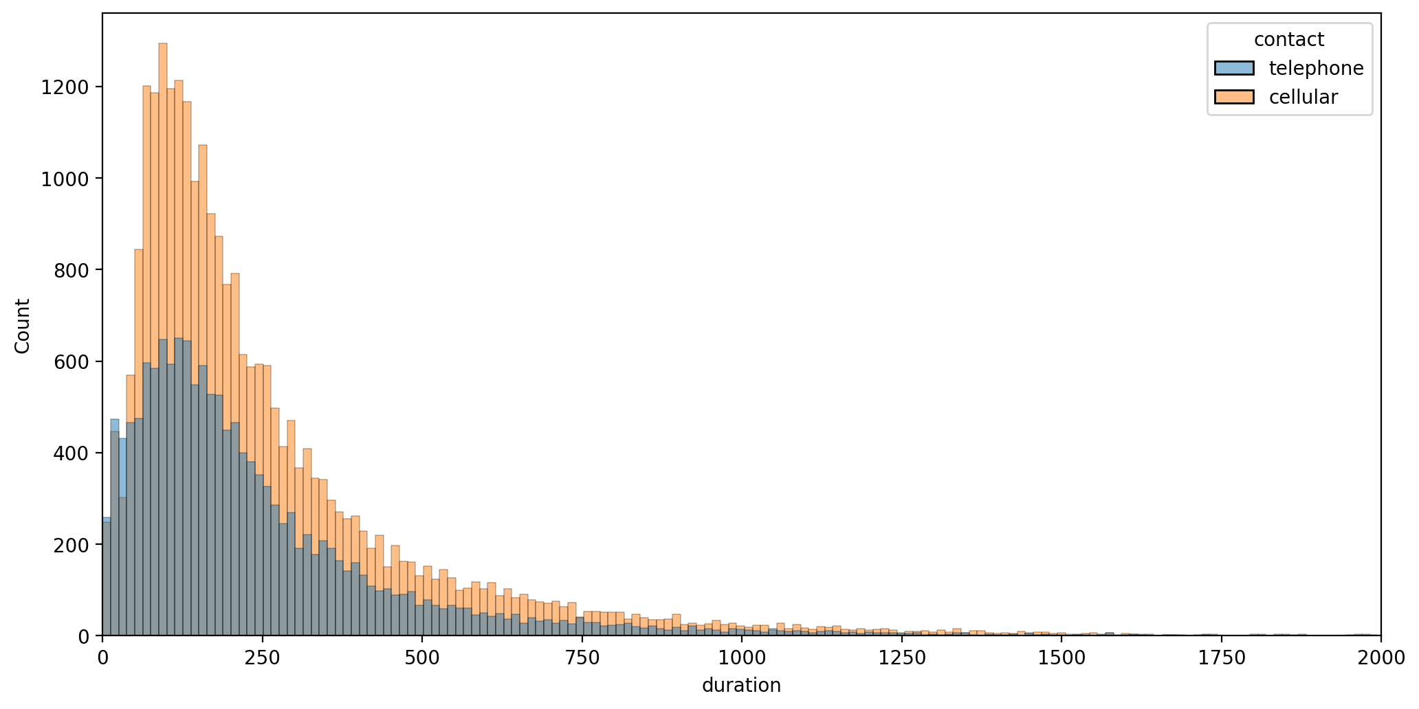

PLOT

• 15 - previous: number of contacts performed before this campaign and for this client (numeric)
• 16 - poutcome: outcome of the previous marketing campaign (categorical: "unknown","other","failure","success"

plt.figure(figsize=(12,6),dpi=200)
sns.countplot(data=df,x='previous',hue='contact')

<AxesSubplot:xlabel='previous', ylabel='count'>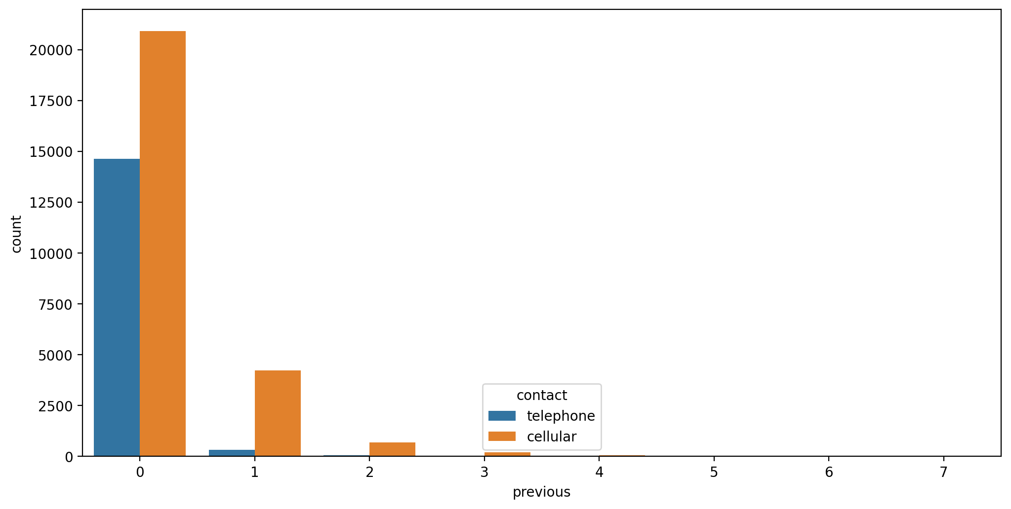

PLOT

sns.countplot(data=df,x='contact')

<AxesSubplot:xlabel='contact', ylabel='count'>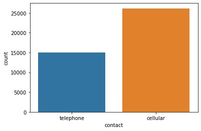

PLOT

# df['previous'].value_counts()
df['previous'].value_counts().sum()-36954
# 36954 vs. 8257

4234

Categorical Features

df.head()

age
job
marital
education
default

plt.figure(figsize=(12,6),dpi=200)
# https://stackoverflow.com/questions/46623583/seaborn-countplot-order-categories-by-count
sns.countplot(data=df,x='job',order=df['job'].value_counts().index)
plt.xticks(rotation=90);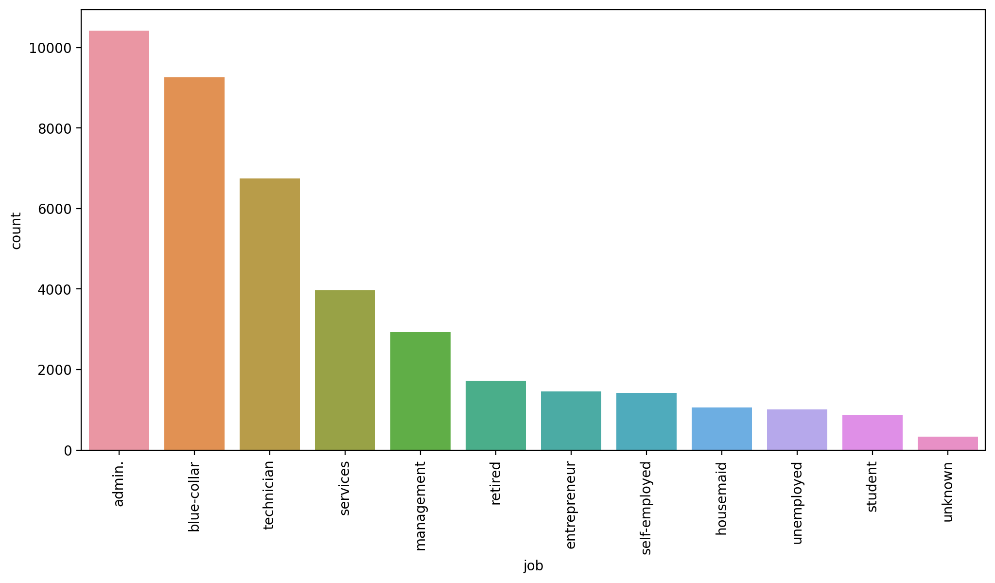

PLOT

plt.figure(figsize=(12,6),dpi=200)
# https://stackoverflow.com/questions/46623583/seaborn-countplot-order-categories-by-count
sns.countplot(data=df,x='education',order=df['education'].value_counts().index)
plt.xticks(rotation=90);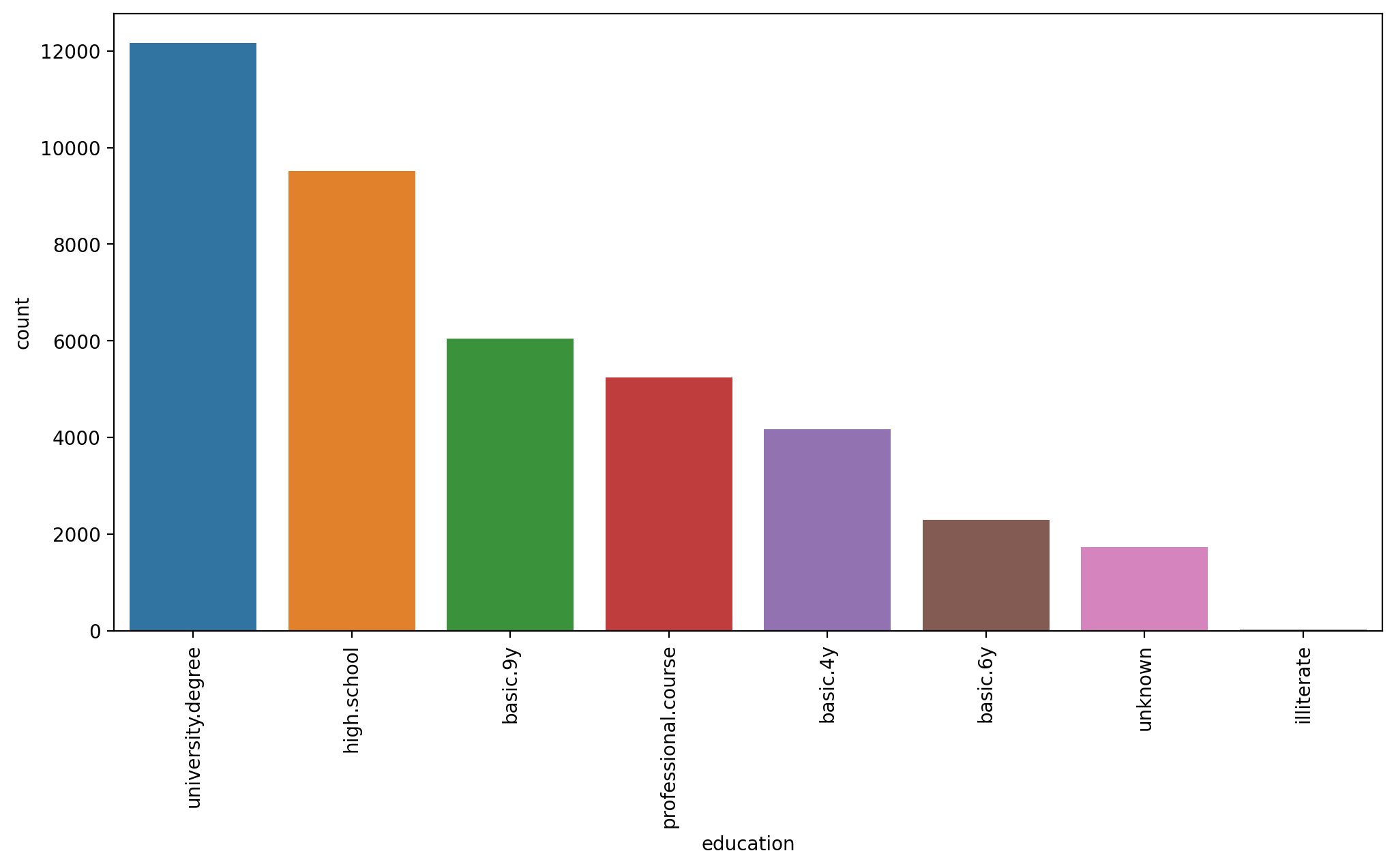

PLOT

plt.figure(figsize=(12,6),dpi=200)
# https://stackoverflow.com/questions/46623583/seaborn-countplot-order-categories-by-count
sns.countplot(data=df,x='education',order=df['education'].value_counts().index,hue='default')
plt.xticks(rotation=90);

PLOT

sns.countplot(data=df,x='default')

<AxesSubplot:xlabel='default', ylabel='count'>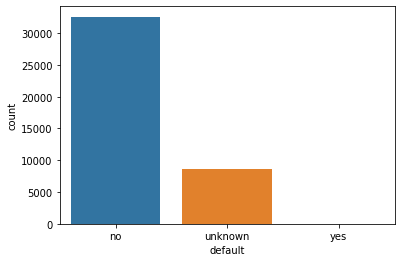

PLOT

# THIS TAKES A LONG TIME!
sns.pairplot(df)

<seaborn.axisgrid.PairGrid at 0x209136c9490>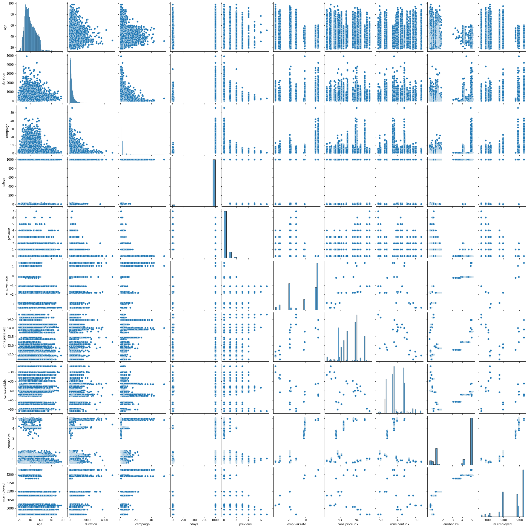

PLOT

Clustering

Data Preparation

UNSUPERVISED LEARNING REMINDER: NO NEED TO TRAIN TEST SPLIT!! NO LABEL TO "TEST" AGAINST!

We do however need to transform categorical features into numeric ones where it makes sense to do so, as well as scaling the data due to distance being a key factor in clustering.

df.head()

age
job
marital
education
default

X = pd.get_dummies(df)

X

age
duration
campaign
pdays
previous

from sklearn.preprocessing import StandardScaler

scaler = StandardScaler()

scaled_X = scaler.fit_transform(X)

Creating and Fitting a KMeans Model

Note of our method choices here:

• fit(X[, y, sample_weight])

  • Compute k-means clustering.

• fit_predict(X[, y, sample_weight])

  • Compute cluster centers and predict cluster index for each sample.

• fit_transform(X[, y, sample_weight])

  • Compute clustering and transform X to cluster-distance space.

• predict(X[, sample_weight])

  • Predict the closest cluster each sample in X belongs to.

from sklearn.cluster import KMeans

model = KMeans(n_clusters=2)

# Make sure to watch video to understand this line and fit() vs transform()
cluster_labels = model.fit_predict(scaled_X)

# IMPORTANT NOTE: YOUR 0s and 1s may be opposite of ours,
# makes sense, the number values are not significant!
cluster_labels

array([0, 0, 0, ..., 1, 1, 1])

len(scaled_X)

41188

len(cluster_labels)

41188

X['Cluster'] = cluster_labels

sns.heatmap(X.corr())

<AxesSubplot:>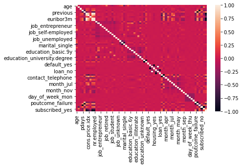

PLOT

X.corr()['Cluster']

age                    -0.019767
duration                0.039581
campaign               -0.129103
pdays                  -0.267714
previous                0.478493

plt.figure(figsize=(12,6),dpi=200)
X.corr()['Cluster'].iloc[:-1].sort_values().plot(kind='bar')

<AxesSubplot:>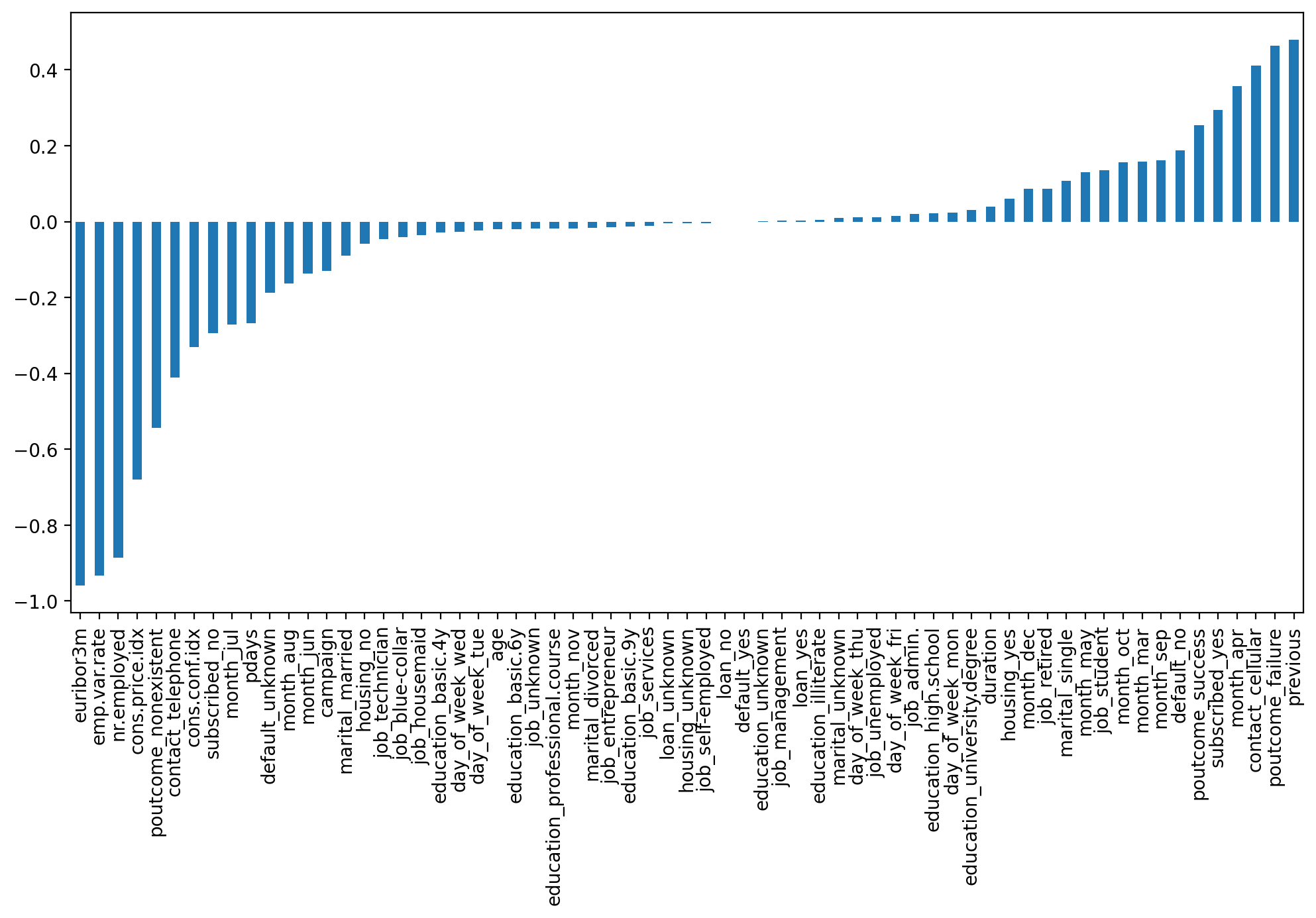

PLOT

Choosing K Value

ssd = []
 
for k in range(2,10):
    
    model = KMeans(n_clusters=k)
    
    
    model.fit(scaled_X)
    
    #Sum of squared distances of samples to their closest cluster center.
    ssd.append(model.inertia_)

plt.plot(range(2,10),ssd,'o--')
plt.xlabel("K Value")
plt.ylabel(" Sum of Squared Distances")

Text(0, 0.5, ' Sum of Squared Distances')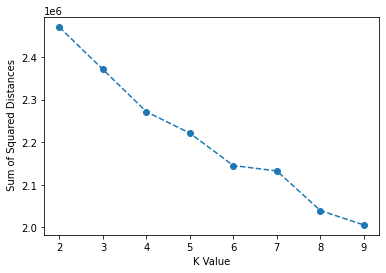

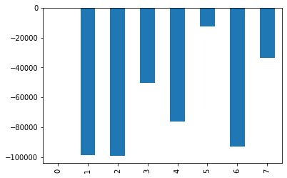
PLOT

Analyzing SSE Reduction

ssd

[2469792.4095956706,
 2370787.709348152,
 2271502.7007717513,
 2221128.900236805,
 2145067.141554143,

# Change in SSD from previous K value!
pd.Series(ssd).diff()

0             NaN
1   -99004.700248
2   -99285.008576
3   -50373.800535
4   -76061.758683

pd.Series(ssd).diff().plot(kind='bar')

<AxesSubplot:>

PLOT