++++

Data Science

May 2026×Notebook lesson

Notebook converted from Jupyter for blog publishing.

03-DBSCAN-Project-Solutions

Driptanil DattaSoftware Developer

DBSCAN Project Solutions

The Data

Source: https://archive.ics.uci.edu/ml/datasets/Wholesale+customers (opens in a new tab)

Margarida G. M. S. Cardoso, margarida.cardoso '@' iscte.pt, ISCTE-IUL, Lisbon, Portugal

Data Set Information:

Provide all relevant information about your data set.

Attribute Information:

1. FRESH: annual spending (m.u.) on fresh products (Continuous);
2. MILK: annual spending (m.u.) on milk products (Continuous);
3. GROCERY: annual spending (m.u.)on grocery products (Continuous);
4. FROZEN: annual spending (m.u.)on frozen products (Continuous)
5. DETERGENTS_PAPER: annual spending (m.u.) on detergents and paper products (Continuous)
6. DELICATESSEN: annual spending (m.u.)on and delicatessen products (Continuous);
7. CHANNEL: customers Channel - Horeca (Hotel/Restaurant/Café) or Retail channel (Nominal)
8. REGION: customers Region Lisnon, Oporto or Other (Nominal)

Relevant Papers:

Cardoso, Margarida G.M.S. (2013). Logical discriminant models – Chapter 8 in Quantitative Modeling in Marketing and Management Edited by Luiz Moutinho and Kun-Huang Huarng. World Scientific. p. 223-253. ISBN 978-9814407717

Jean-Patrick Baudry, Margarida Cardoso, Gilles Celeux, Maria José Amorim, Ana Sousa Ferreira (2012). Enhancing the selection of a model-based clustering with external qualitative variables. RESEARCH REPORT N° 8124, October 2012, Project-Team SELECT. INRIA Saclay - Île-de-France, Projet select, Université Paris-Sud 11

DBSCAN and Clustering Examples

COMPLETE THE TASKS IN BOLD BELOW:

TASK: Run the following cells to import the data and view the DataFrame.

import numpy as np
import pandas as pd
import matplotlib.pyplot as plt
import seaborn as sns

df = pd.read_csv('../DATA/wholesome_customers_data.csv')

df.head()

Channel
Region
Fresh
Milk
Grocery

df.info()

<class 'pandas.core.frame.DataFrame'>
RangeIndex: 440 entries, 0 to 439
Data columns (total 8 columns):
 #   Column            Non-Null Count  Dtype
---  ------            --------------  -----

EDA

TASK: Create a scatterplot showing the relation between MILK and GROCERY spending, colored by Channel column.

#CODE HERE

sns.scatterplot(data=df,x='Milk',y='Grocery',hue='Channel')

<AxesSubplot:xlabel='Milk', ylabel='Grocery'>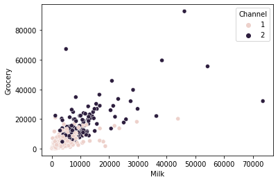

PLOT

TASK: Use seaborn to create a histogram of MILK spending, colored by Channel. Can you figure out how to use seaborn to "stack" the channels, instead of have them overlap?

#CODE HERE

sns.histplot(df,x='Milk',hue='Channel',multiple="stack")

<AxesSubplot:xlabel='Milk', ylabel='Count'>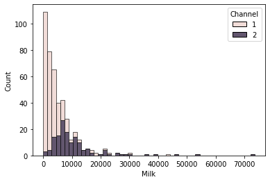

PLOT

TASK: Create an annotated clustermap of the correlations between spending on different cateogires.

# CODE HERE

print('Correlation Between Spending Categories')
sns.clustermap(df.drop(['Region','Channel'],axis=1).corr(),annot=True);

Correlation Between Spending Categories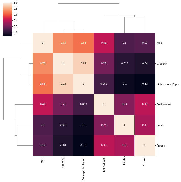

PLOT

TASK: Create a PairPlot of the dataframe, colored by Region.

#CODE HERE

sns.pairplot(df,hue='Region',palette='Set1')

<seaborn.axisgrid.PairGrid at 0x2d711759c40>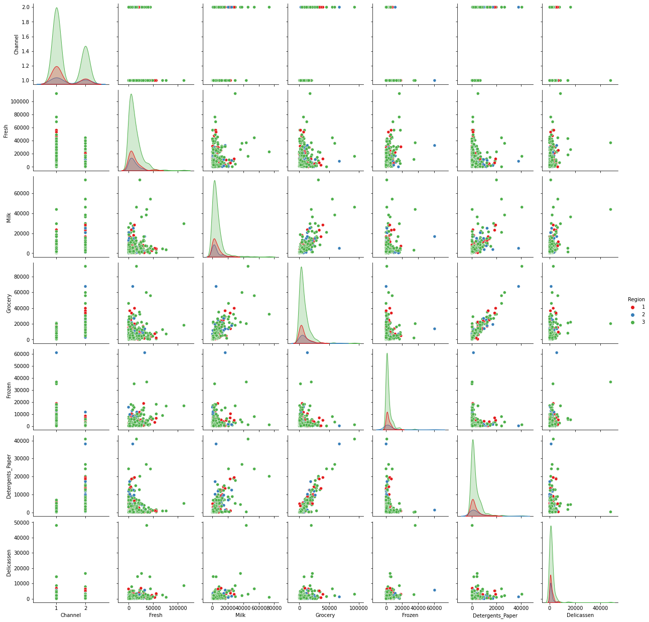

PLOT

DBSCAN

TASK: Since the values of the features are in different orders of magnitude, let's scale the data. Use StandardScaler to scale the data.

#CODE HERE

from sklearn.preprocessing import StandardScaler
scaler = StandardScaler()
scaled_X = scaler.fit_transform(df)

scaled_X

array([[ 1.44865163,  0.59066829,  0.05293319, ..., -0.58936716,
        -0.04356873, -0.06633906],
       [ 1.44865163,  0.59066829, -0.39130197, ..., -0.27013618,
         0.08640684,  0.08915105],
       [ 1.44865163,  0.59066829, -0.44702926, ..., -0.13753572,

TASK: Use DBSCAN and a for loop to create a variety of models testing different epsilon values. Set min_samples equal to 2 times the number of features. During the loop, keep track of and log the percentage of points that are outliers. For reference the solutions notebooks uses the following range of epsilon values for testing:

np.linspace(0.001,3,50)

#CODE HERE

from sklearn.cluster import DBSCAN

outlier_percent = []
 
for eps in np.linspace(0.001,3,50):
    
    # Create Model
    dbscan = DBSCAN(eps=eps,min_samples=2*scaled_X.shape[1])
    dbscan.fit(scaled_X)
   
     
    # Log percentage of points that are outliers
    perc_outliers = 100 * np.sum(dbscan.labels_ == -1) / len(dbscan.labels_)
    
    outlier_percent.append(perc_outliers)

TASK: Create a line plot of the percentage of outlier points versus the epsilon value choice.

#CODE HERE

sns.lineplot(x=np.linspace(0.001,3,50),y=outlier_percent)
plt.ylabel("Percentage of Points Classified as Outliers")
plt.xlabel("Epsilon Value")

Text(0.5, 0, 'Epsilon Value')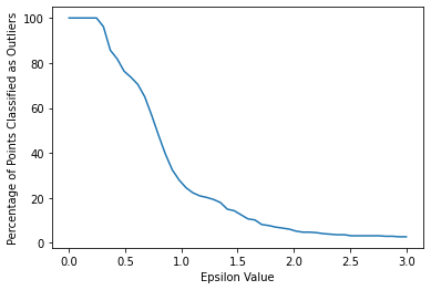

PLOT

DBSCAN with Chosen Epsilon

TASK: Based on the plot created in the previous task, retrain a DBSCAN model with a reasonable epsilon value. Note: For reference, the solutions use eps=2.

dbscan = DBSCAN(eps=2)
dbscan.fit(scaled_X)

DBSCAN(eps=2)

TASK: Create a scatterplot of Milk vs Grocery, colored by the discovered labels of the DBSCAN model.

#CODE HERE

sns.scatterplot(data=df,x='Grocery',y='Milk',hue=dbscan.labels_)

<AxesSubplot:xlabel='Grocery', ylabel='Milk'>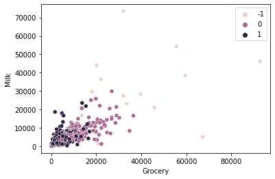

PLOT

TASK: Create a scatterplot of Milk vs. Detergents Paper colored by the labels.

#CODE HERE

sns.scatterplot(data=df,x='Detergents_Paper',y='Milk',hue=dbscan.labels_)

<AxesSubplot:xlabel='Detergents_Paper', ylabel='Milk'>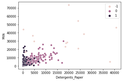

PLOT

TASK: Create a new column on the original dataframe called "Labels" consisting of the DBSCAN labels.

#CODE HERE

df['Labels'] = dbscan.labels_

df.head()

Channel
Region
Fresh
Milk
Grocery

TASK: Compare the statistical mean of the clusters and outliers for the spending amounts on the categories.

# CODE HERE

cats = df.drop(['Channel','Region'],axis=1)
cat_means = cats.groupby('Labels').mean()

cat_means

Fresh
Milk
Grocery
Frozen
Detergents_Paper

TASK: Normalize the dataframe from the previous task using MinMaxScaler so the spending means go from 0-1 and create a heatmap of the values.

#CODE HERE

from sklearn.preprocessing import MinMaxScaler

scaler = MinMaxScaler()
data = scaler.fit_transform(cat_means)
scaled_means = pd.DataFrame(data,cat_means.index,cat_means.columns)

scaled_means

Fresh
Milk
Grocery
Frozen
Detergents_Paper

sns.heatmap(scaled_means)

<AxesSubplot:ylabel='Labels'>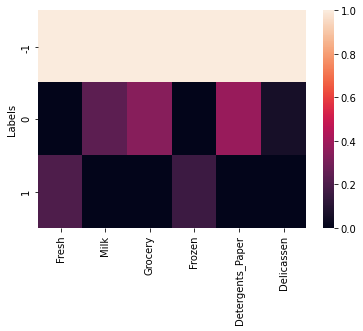

PLOT

TASK: Create another heatmap similar to the one above, but with the outliers removed

sns.heatmap(scaled_means.loc[[0,1]],annot=True)

<AxesSubplot:ylabel='Labels'>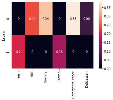

PLOT

TASK: What spending category were the two clusters mode different in?

#CODE HERE

We can see that Detergents Paper was the most significant difference.