++++

Data Science

May 2026×Notebook lesson

Notebook converted from Jupyter for blog publishing.

01-SVM-Regression

Driptanil DattaSoftware Developer

Support Vector Machines

SVM - Regression

The concrete slump test measures the consistency of fresh concrete before it sets. It is performed to check the workability of freshly made concrete, and therefore the ease with which concrete flows. It can also be used as an indicator of an improperly mixed batch.

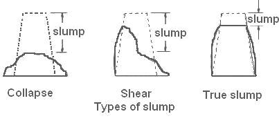
Our data set consists of various cement properties and the resulting slump test metrics in cm. Later on the set concrete is tested for its compressive strength 28 days later.

Input variables (7)(component kg in one M^3 concrete):

• Cement
• Slag
• Fly ash
• Water
• SP
• Coarse Aggr.
• Fine Aggr.

Output variables (3):

• SLUMP (cm)
• FLOW (cm)
• 28-day Compressive Strength (Mpa)

Data Source: https://archive.ics.uci.edu/ml/datasets/Concrete+Slump+Test (opens in a new tab)

Credit: Yeh, I-Cheng, "Modeling slump flow of concrete using second-order regressions and artificial neural networks," Cement and Concrete Composites, Vol.29, No. 6, 474-480, 2007.

import numpy as np
import pandas as pd
import seaborn as sns
import matplotlib.pyplot as plt

df = pd.read_csv('../DATA/cement_slump.csv')

df.head()

Cement
Slag
Fly ash
Water
SP

df.corr()['Compressive Strength (28-day)(Mpa)']

Cement                                0.445656
Slag                                 -0.331522
Fly ash                               0.444380
Water                                -0.254320
SP                                   -0.037909

plt.figure(figsize=(10, 6), dpi=100)
sns.heatmap(df.corr(), annot=True)

<Axes: >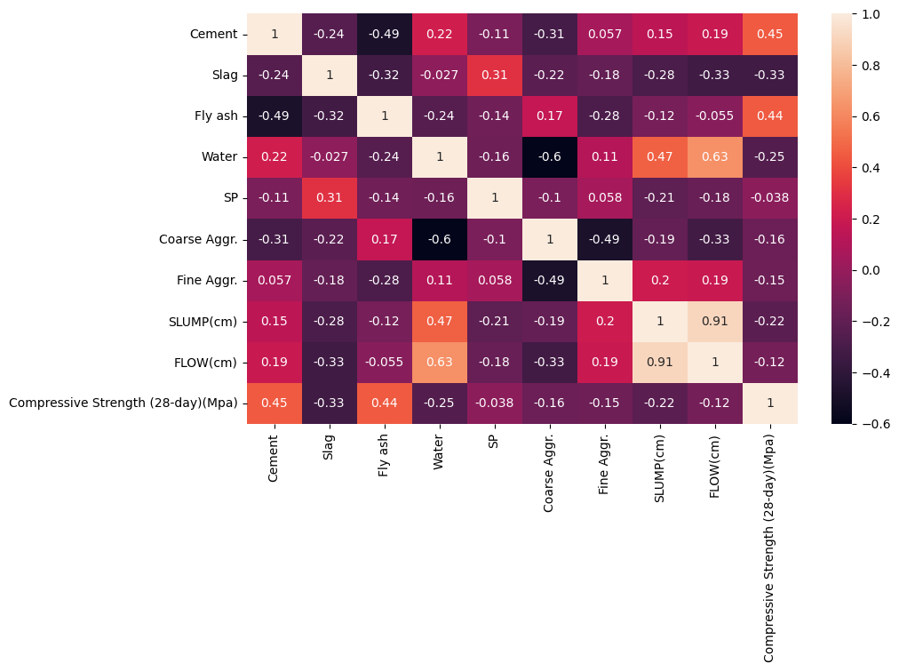

PLOT

df.columns

Index(['Cement', 'Slag', 'Fly ash', 'Water', 'SP', 'Coarse Aggr.',
       'Fine Aggr.', 'SLUMP(cm)', 'FLOW(cm)',
       'Compressive Strength (28-day)(Mpa)'],
      dtype='object')

Train | Test Split

Alternatively you could also set this up as a pipline, something like:

from sklearn.pipeline import make_pipeline from sklearn.preprocessing import StandardScaler from sklearn.svm import SVR

clf = make_pipeline(StandardScaler(), SVR())

df.columns

Index(['Cement', 'Slag', 'Fly ash', 'Water', 'SP', 'Coarse Aggr.',
       'Fine Aggr.', 'SLUMP(cm)', 'FLOW(cm)',
       'Compressive Strength (28-day)(Mpa)'],
      dtype='object')

X = df.drop('Compressive Strength (28-day)(Mpa)',axis=1)
y = df['Compressive Strength (28-day)(Mpa)']

from sklearn.model_selection import train_test_split

X_train, X_test, y_train, y_test = train_test_split(X, y, test_size=0.3, random_state=101)

from sklearn.preprocessing import StandardScaler

scaler = StandardScaler()

scaled_X_train = scaler.fit_transform(X_train)
scaled_X_test = scaler.transform(X_test)

Support Vector Machines - Regression

There are three different implementations of Support Vector Regression: SVR, NuSVR and LinearSVR. LinearSVR provides a faster implementation than SVR but only considers the linear kernel, while NuSVR implements a slightly different formulation than SVR and LinearSVR. See Implementation details (opens in a new tab) for further details.

from sklearn.svm import SVR,LinearSVR

Setting C: C is 1 by default and it’s a reasonable default choice. If you have a lot of noisy observations you should decrease it: decreasing C corresponds to more regularization.

LinearSVC and LinearSVR are less sensitive to C when it becomes large, and prediction results stop improving after a certain threshold. Meanwhile, larger C values will take more time to train, sometimes up to 10 times longer

Epsilon: https://stats.stackexchange.com/questions/259018/meaning-of-epsilon-in-svm-regression (opens in a new tab)

base_model = SVR()

base_model.fit(scaled_X_train,y_train)

SVR()

base_preds = base_model.predict(scaled_X_test)

Evaluation

from sklearn.metrics import mean_absolute_error,mean_squared_error

mean_absolute_error(y_test,base_preds)

5.236902091259178

np.sqrt(mean_squared_error(y_test,base_preds))

6.695914838327133

y_test.mean()

36.26870967741935

Grid Search in Attempt for Better Model

param_grid = {'C':[0.001,0.01,0.1,0.5,1],
             'kernel':['linear','rbf','poly'],
              'gamma':['scale','auto'],
              'degree':[2,3,4],
              'epsilon':[0,0.01,0.1,0.5,1,2]}

from sklearn.model_selection import GridSearchCV

svr = SVR()
grid = GridSearchCV(svr,param_grid=param_grid)

grid.fit(scaled_X_train,y_train)

GridSearchCV(estimator=SVR(),
             param_grid={'C': [0.001, 0.01, 0.1, 0.5, 1], 'degree': [2, 3, 4],
                         'epsilon': [0, 0.01, 0.1, 0.5, 1, 2],
                         'gamma': ['scale', 'auto'],
                         'kernel': ['linear', 'rbf', 'poly']})

grid.best_params_

{'C': 1, 'degree': 2, 'epsilon': 2, 'gamma': 'scale', 'kernel': 'linear'}

grid_preds = grid.predict(scaled_X_test)

mean_absolute_error(y_test,grid_preds)

2.5128012210762365

np.sqrt(mean_squared_error(y_test,grid_preds))

3.178210305119858

Great improvement!