 ++++
++++Notebook converted from Jupyter for blog publishing.
00-KNN-Classification
KNN - K Nearest Neighbors - Classification
To understand KNN for classification, we'll work with a simple dataset representing gene expression levels. Gene expression levels are calculated by the ratio between the expression of the target gene (i.e., the gene of interest) and the expression of one or more reference genes (often household genes). This dataset is synthetic and specifically designed to show some of the strengths and limitations of using KNN for Classification.
More info on gene expression: https://www.sciencedirect.com/topics/biochemistry-genetics-and-molecular-biology/gene-expression-level (opens in a new tab)
Imports
import numpy as np
import pandas as pd
import matplotlib.pyplot as plt
import seaborn as sns
Data
df = pd.read_csv('../DATA/gene_expression.csv')df.head()Gene One
Gene Two
Cancer Present
0
4.3sns.scatterplot(x='Gene One',y='Gene Two',hue='Cancer Present',data=df,alpha=0.7)<Axes: xlabel='Gene One', ylabel='Gene Two'>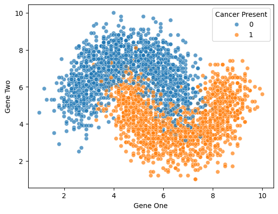
sns.scatterplot(x='Gene One',y='Gene Two',hue='Cancer Present',data=df)
plt.xlim(2,6)
plt.ylim(3,10)
# plt.legend(loc=(1.1,0.5))(3.0, 10.0)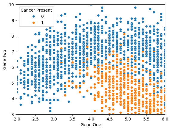
Train|Test Split and Scaling Data
from sklearn.model_selection import train_test_split
from sklearn.preprocessing import StandardScaler
X = df.drop('Cancer Present',axis=1)
y = df['Cancer Present']X_train, X_test, y_train, y_test = train_test_split(X, y, test_size=0.3, random_state=42)NameError: name 'train_test_split' is not defined
---------------------------------------------------------------------------
NameError Traceback (most recent call last)
Cell In[3], line 1
----> 1 X_train, X_test, y_train, y_test = train_test_split(X, y, test_size=0.3, random_state=42)scaler = StandardScaler()scaled_X_train = scaler.fit_transform(X_train)
scaled_X_test = scaler.transform(X_test)from sklearn.neighbors import KNeighborsClassifierknn_model = KNeighborsClassifier(n_neighbors=1)knn_model.fit(scaled_X_train,y_train)KNeighborsClassifier(n_neighbors=1)Understanding KNN and Choosing K Value
full_test = pd.concat([X_test,y_test],axis=1)len(full_test)900sns.scatterplot(x='Gene One',y='Gene Two',hue='Cancer Present',
data=full_test,alpha=0.7)<AxesSubplot:xlabel='Gene One', ylabel='Gene Two'>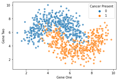
Model Evaluation
y_pred = knn_model.predict(scaled_X_test)from sklearn.metrics import classification_report,confusion_matrix,accuracy_scoreaccuracy_score(y_test,y_pred)0.8922222222222222confusion_matrix(y_test,y_pred)array([[420, 50],
[ 47, 383]], dtype=int64)print(classification_report(y_test,y_pred)) precision recall f1-score support
0 0.90 0.89 0.90 470
1 0.88 0.89 0.89 430
Elbow Method for Choosing Reasonable K Values
NOTE: This uses the test set for the hyperparameter selection of K.
test_error_rates = []


for k in range(1,30):
    knn_model = KNeighborsClassifier(n_neighbors=k)
    knn_model.fit(scaled_X_train,y_train)

    y_pred_test = knn_model.predict(scaled_X_test)

    test_error = 1 - accuracy_score(y_test,y_pred_test)
test_error_rates.append(test_error)plt.figure(figsize=(10,6),dpi=200)
plt.plot(range(1,30),test_error_rates,label='Test Error')
plt.legend()
plt.ylabel('Error Rate')
plt.xlabel("K Value")Text(0.5, 0, 'K Value')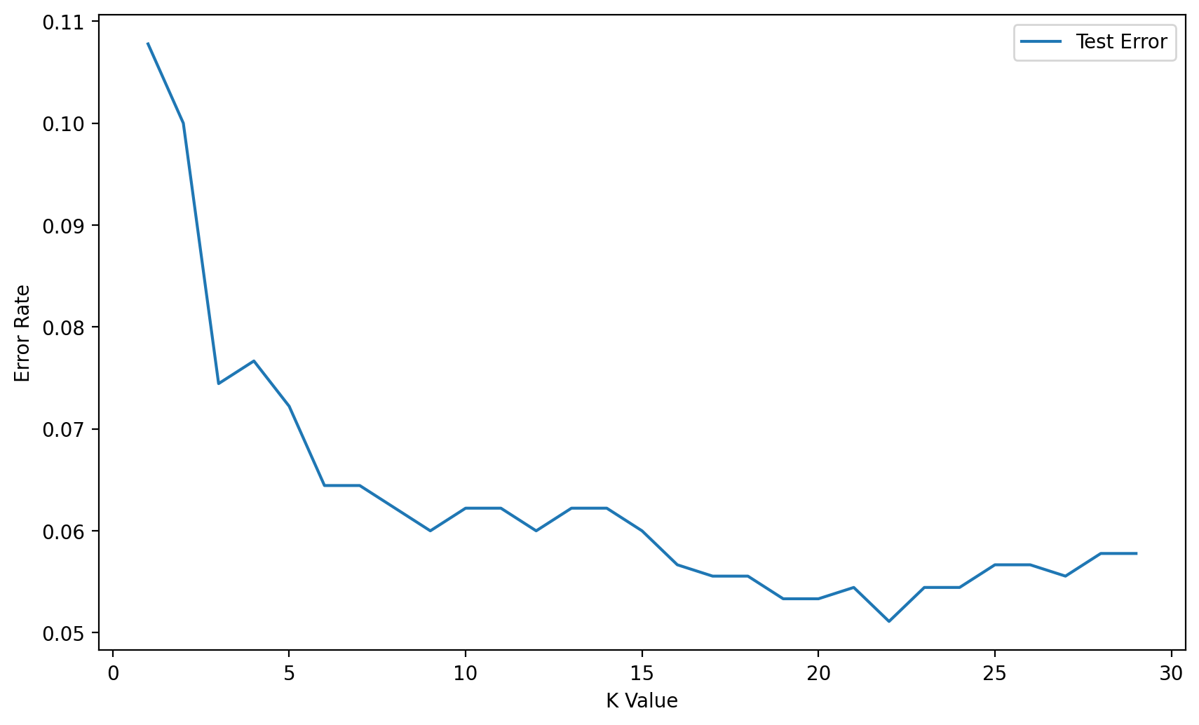
Full Cross Validation Grid Search for K Value
Creating a Pipeline to find K value
Follow along very carefully here! We use very specific string codes AND variable names here so that everything matches up correctly. This is not a case where you can easily swap out variable names for whatever you want!
We'll use a Pipeline object to set up a workflow of operations:
- Scale Data
- Create Model on Scaled Data
How does the Scaler work inside a Pipeline with CV? Is scikit-learn "smart" enough to understand .fit() on train vs .transform() on train and test?*
**Yes! Scikit-Learn's pipeline is well suited for this! Full Info in Documentation (opens in a new tab) **
When you use the StandardScaler as a step inside a Pipeline then scikit-learn will internally do the job for you.
What happens can be discribed as follows:
- Step 0: The data are split into TRAINING data and TEST data according to the cv parameter that you specified in the GridSearchCV.
- Step 1: the scaler is fitted on the TRAINING data
- Step 2: the scaler transforms TRAINING data
- Step 3: the models are fitted/trained using the transformed TRAINING data
- Step 4: the scaler is used to transform the TEST data
- Step 5: the trained models predict using the transformed TEST data
scaler = StandardScaler()knn = KNeighborsClassifier()knn.get_params().keys()dict_keys(['algorithm', 'leaf_size', 'metric', 'metric_params', 'n_jobs', 'n_neighbors', 'p', 'weights'])# Highly recommend string code matches variable name!
operations = [('scaler',scaler),('knn',knn)]from sklearn.pipeline import Pipelinepipe = Pipeline(operations)from sklearn.model_selection import GridSearchCVNote: If your parameter grid is going inside a PipeLine, your parameter name needs to be specified in the following manner:*
- chosen_string_name + two underscores + parameter key name
- model_name + __ + parameter name
- knn_model + __ + n_neighbors
- knn_model__n_neighbors
StackOverflow on this (opens in a new tab)
The reason we have to do this is because it let's scikit-learn know what operation in the pipeline these parameters are related to (otherwise it might think n_neighbors was a parameter in the scaler).
k_values = list(range(1,20))k_values[1, 2, 3, 4, 5, 6, 7, 8, 9, 10, 11, 12, 13, 14, 15, 16, 17, 18, 19]
param_grid = {'knn__n_neighbors': k_values}full_cv_classifier = GridSearchCV(pipe,param_grid,cv=5,scoring='accuracy')# Use full X and y if you DON'T want a hold-out test set
# Use X_train and y_train if you DO want a holdout test set (X_test,y_test)
full_cv_classifier.fit(X_train,y_train)GridSearchCV(cv=5,
estimator=Pipeline(steps=[('scaler', StandardScaler()),
('knn', KNeighborsClassifier())]),
param_grid={'knn__n_neighbors': [1, 2, 3, 4, 5, 6, 7, 8, 9, 10, 11,
12, 13, 14, 15, 16, 17, 18, 19]},full_cv_classifier.best_estimator_.get_params(){'memory': None,
'steps': [('scaler', StandardScaler()),
('knn', KNeighborsClassifier(n_neighbors=14))],
'verbose': False,
'scaler': StandardScaler(),full_cv_classifier.cv_results_.keys()dict_keys(['mean_fit_time', 'std_fit_time', 'mean_score_time', 'std_score_time', 'param_knn__n_neighbors', 'params', 'split0_test_score', 'split1_test_score', 'split2_test_score', 'split3_test_score', 'split4_test_score', 'mean_test_score', 'std_test_score', 'rank_test_score'])Let's check our understanding: How many total runs did we do?
len(k_values)19full_cv_classifier.cv_results_['mean_test_score']array([0.90238095, 0.90285714, 0.91857143, 0.91333333, 0.92380952,
0.92142857, 0.9252381 , 0.9247619 , 0.9252381 , 0.92190476,
0.9252381 , 0.9247619 , 0.92761905, 0.92904762, 0.92809524,
0.92809524, 0.92904762, 0.92857143, 0.92761905])len(full_cv_classifier.cv_results_['mean_test_score'])19Final Model
We just saw that our GridSearch recommends a K=14 (in line with our alternative Elbow Method). Let's now use the PipeLine again, but this time, no need to do a grid search, instead we will evaluate on our hold-out Test Set.
scaler = StandardScaler()
knn14 = KNeighborsClassifier(n_neighbors=14)
operations = [('scaler',scaler),('knn14',knn14)]
pipe = Pipeline(operations)pipe.fit(X_train,y_train)Pipeline(steps=[('scaler', StandardScaler()),
('knn14', KNeighborsClassifier(n_neighbors=14))])pipe_pred = pipe.predict(X_test)print(classification_report(y_test,pipe_pred)) precision recall f1-score support
0 0.93 0.95 0.94 470
1 0.95 0.92 0.93 430
single_sample = X_test.iloc[40]single_sampleGene One 3.8
Gene Two 6.3
Name: 194, dtype: float64pipe.predict(single_sample.values.reshape(1, -1))array([0], dtype=int64)pipe.predict_proba(single_sample.values.reshape(1, -1))array([[0.92857143, 0.07142857]])