++++

Data Science

May 2026×Notebook lesson

Notebook converted from Jupyter for blog publishing.

00-SVM-Classification

Driptanil DattaSoftware Developer

Exploring Support Vector Machines

NOTE: For this example, we will explore the algorithm, so we'll skip scaling and also skip a train\test split and instead see how the various parameters can change an SVM (easiest to visualize the effects in classification)

Link to a great Paper on SVM (opens in a new tab)

• A tutorial on support vector regression by ALEX J. SMOLA and BERNHARD SCHOLKOPF

SVM - Classification

import numpy as np
import pandas as pd
import seaborn as sns
import matplotlib.pyplot as plt

Data

The data shown here simulates a medical study in which mice infected with a virus were given various doses of two medicines and then checked 2 weeks later to see if they were still infected. Given this data, our goal is to create a classifcation model than predict (given two dosage measurements) if they mouse will still be infected with the virus.

You will notice the groups are very separable, this is on purpose, to explore how the various parameters of an SVM model behave.

df = pd.read_csv("../DATA/mouse_viral_study.csv")

df.head()

Med_1_mL
Med_2_mL
Virus Present
0
6.508231

df.columns

Index(['Med_1_mL', 'Med_2_mL', 'Virus Present'], dtype='object')

Classes

sns.scatterplot(x='Med_1_mL',y='Med_2_mL',hue='Virus Present',
                data=df,palette='seismic')

<AxesSubplot:xlabel='Med_1_mL', ylabel='Med_2_mL'>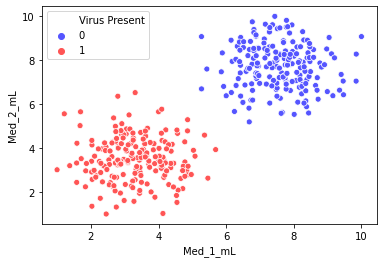

PLOT

Separating Hyperplane

Our goal with SVM is to create the best separating hyperplane. In 2 dimensions, this is simply a line.

sns.scatterplot(x='Med_1_mL',y='Med_2_mL',hue='Virus Present',palette='seismic',data=df)
 
# We want to somehow automatically create a separating hyperplane ( a line in 2D)
 
x = np.linspace(0,10,100)
m = -1
b = 11
y = m*x + b
plt.plot(x,y,'k')

[<matplotlib.lines.Line2D at 0x1dab706f208>]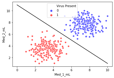

PLOT

SVM - Support Vector Machine

from sklearn.svm import SVC # Supprt Vector Classifier

help(SVC)

Help on class SVC in module sklearn.svm._classes:

class SVC(sklearn.svm._base.BaseSVC)
 |  SVC(*, C=1.0, kernel='rbf', degree=3, gamma='scale', coef0=0.0, shrinking=True, probability=False, tol=0.001, cache_size=200, class_weight=None, verbose=False, max_iter=-1, decision_function_shape='ovr', break_ties=False, random_state=None)
 |  

NOTE: For this example, we will explore the algorithm, so we'll skip any scaling or even a train\test split for now

y = df['Virus Present']
X = df.drop('Virus Present',axis=1)

model = SVC(kernel='linear', C=1000)
model.fit(X, y)

SVC(C=1000, kernel='linear')

# This is imported from the supplemental .py file
# https://scikit-learn.org/stable/auto_examples/svm/plot_separating_hyperplane.html
from svm_margin_plot import plot_svm_boundary

plot_svm_boundary(model,X,y)

PLOT

Hyper Parameters

C

Regularization parameter. The strength of the regularization is inversely proportional to C. Must be strictly positive. The penalty is a squared l2 penalty.

Note: If you are following along with the equations, specifically the value of C as described in ISLR, C in scikit-learn is inversely proportional to this value.

model = SVC(kernel='linear', C=0.05)
model.fit(X, y)

SVC(C=0.05, kernel='linear')

plot_svm_boundary(model,X,y)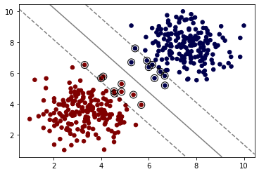

PLOT

Kernel

Choosing a Kernel (opens in a new tab)

rbf - Radial Basis Function (opens in a new tab)

When training an SVM with the Radial Basis Function (RBF) kernel, two parameters must be considered: C and gamma. The parameter C, common to all SVM kernels, trades off misclassification of training examples against simplicity of the decision surface. A low C makes the decision surface smooth, while a high C aims at classifying all training examples correctly. gamma defines how much influence a single training example has. The larger gamma is, the closer other examples must be to be affected.

model = SVC(kernel='rbf', C=1)
model.fit(X, y)
plot_svm_boundary(model,X,y)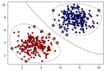

PLOT

model = SVC(kernel='sigmoid')
model.fit(X, y)
plot_svm_boundary(model,X,y)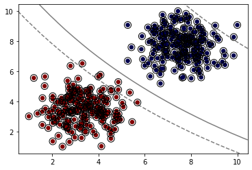

PLOT

Degree (poly kernels only)

Degree of the polynomial kernel function ('poly'). Ignored by all other kernels.

model = SVC(kernel='poly', C=1,degree=1)
model.fit(X, y)
plot_svm_boundary(model,X,y)

PLOT

model = SVC(kernel='poly', C=1,degree=2)
model.fit(X, y)
plot_svm_boundary(model,X,y)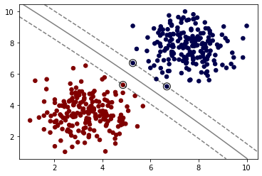

PLOT

gamma

gamma : {'scale', 'auto'} or float, default='scale' Kernel coefficient for 'rbf', 'poly' and 'sigmoid'.

• if gamma='scale'{:python} (default) is passed then it uses 1 / (n_features * X.var()) as value of gamma,
• if 'auto', uses 1 / n_features.

model = SVC(kernel='rbf', C=1,gamma=0.01)
model.fit(X, y)
plot_svm_boundary(model,X,y)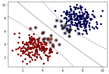

PLOT

Grid Search

Keep in mind, for this simple example, we saw the classes were easily separated, which means each variation of model could easily get 100% accuracy, meaning a grid search is "useless".

from sklearn.model_selection import GridSearchCV

svm = SVC()
param_grid = {'C':[0.01,0.1,1],'kernel':['linear','rbf']}
grid = GridSearchCV(svm,param_grid)

# Note again we didn't split Train|Test
grid.fit(X,y)

GridSearchCV(estimator=SVC(),
             param_grid={'C': [0.01, 0.1, 1, 10], 'kernel': ['linear', 'rbf']})

# 100% accuracy (as expected)
grid.best_score_

1.0

grid.best_params_

{'C': 0.01, 'kernel': 'linear'}

This is more to review the grid search process, recall in a real situation such as your exercise, you will perform a train|test split and get final evaluation metrics.