++++

Data Science

May 2026×Notebook lesson

Notebook converted from Jupyter for blog publishing.

00-PCA-Manual-Implementation

Driptanil DattaSoftware Developer

Principal Component Analysis

Imports

import numpy as np 
import pandas as pd
import matplotlib.pyplot as plt
import seaborn as sns

Data

Breast cancer wisconsin (diagnostic) dataset

Data Set Characteristics:

:Number of Instances: 569

:Number of Attributes: 30 numeric, predictive attributes and the class

:Attribute Information:

radius (mean of distances from center to points on the perimeter)
texture (standard deviation of gray-scale values)
perimeter
area
smoothness (local variation in radius lengths)
compactness (perimeter^2 / area - 1.0)
concavity (severity of concave portions of the contour)
concave points (number of concave portions of the contour)
symmetry
fractal dimension ("coastline approximation" - 1)

The mean, standard error, and "worst" or largest (mean of the three worst/largest values) of these features were computed for each image, resulting in 30 features. For instance, field 0 is Mean Radius, field 10 is Radius SE, field 20 is Worst Radius.

class:
- WDBC-Malignant
- WDBC-Benign

:Summary Statistics:

===================================== ====== ====== Min Max ===================================== ====== ====== radius (mean): 6.981 28.11 texture (mean): 9.71 39.28 perimeter (mean): 43.79 188.5 area (mean): 143.5 2501.0 smoothness (mean): 0.053 0.163 compactness (mean): 0.019 0.345 concavity (mean): 0.0 0.427 concave points (mean): 0.0 0.201 symmetry (mean): 0.106 0.304 fractal dimension (mean): 0.05 0.097 radius (standard error): 0.112 2.873 texture (standard error): 0.36 4.885 perimeter (standard error): 0.757 21.98 area (standard error): 6.802 542.2 smoothness (standard error): 0.002 0.031 compactness (standard error): 0.002 0.135 concavity (standard error): 0.0 0.396 concave points (standard error): 0.0 0.053 symmetry (standard error): 0.008 0.079 fractal dimension (standard error): 0.001 0.03 radius (worst): 7.93 36.04 texture (worst): 12.02 49.54 perimeter (worst): 50.41 251.2 area (worst): 185.2 4254.0 smoothness (worst): 0.071 0.223 compactness (worst): 0.027 1.058 concavity (worst): 0.0 1.252 concave points (worst): 0.0 0.291 symmetry (worst): 0.156 0.664 fractal dimension (worst): 0.055 0.208 ===================================== ====== ======

:Missing Attribute Values: None

:Class Distribution: 212 - Malignant, 357 - Benign

:Creator: Dr. William H. Wolberg, W. Nick Street, Olvi L. Mangasarian

:Donor: Nick Street

:Date: November, 1995

This is a copy of UCI ML Breast Cancer Wisconsin (Diagnostic) datasets. https://goo.gl/U2Uwz2 (opens in a new tab)

Features are computed from a digitized image of a fine needle aspirate (FNA) of a breast mass. They describe characteristics of the cell nuclei present in the image.

Separating plane described above was obtained using Multisurface Method-Tree (MSM-T) [K. P. Bennett, "Decision Tree Construction Via Linear Programming." Proceedings of the 4th Midwest Artificial Intelligence and Cognitive Science Society, pp. 97-101, 1992], a classification method which uses linear programming to construct a decision tree. Relevant features were selected using an exhaustive search in the space of 1-4 features and 1-3 separating planes.

The actual linear program used to obtain the separating plane in the 3-dimensional space is that described in: [K. P. Bennett and O. L. Mangasarian: "Robust Linear Programming Discrimination of Two Linearly Inseparable Sets", Optimization Methods and Software 1, 1992, 23-34].

This database is also available through the UW CS ftp server:

ftp ftp.cs.wisc.edu cd math-prog/cpo-dataset/machine-learn/WDBC/

.. topic:: References

W.N. Street, W.H. Wolberg and O.L. Mangasarian. Nuclear feature extraction for breast tumor diagnosis. IS&T/SPIE 1993 International Symposium on Electronic Imaging: Science and Technology, volume 1905, pages 861-870, San Jose, CA, 1993.
O.L. Mangasarian, W.N. Street and W.H. Wolberg. Breast cancer diagnosis and prognosis via linear programming. Operations Research, 43(4), pages 570-577, July-August 1995.
W.H. Wolberg, W.N. Street, and O.L. Mangasarian. Machine learning techniques to diagnose breast cancer from fine-needle aspirates. Cancer Letters 77 (1994) 163-171.

df = pd.read_csv('../DATA/cancer_tumor_data_features.csv')

df.head()

HTML

mean radius
mean texture
mean perimeter
mean area
mean smoothness

Manual Construction of PCA

Scaling Data

from sklearn.preprocessing import StandardScaler

scaler = StandardScaler()

scaled_X = scaler.fit_transform(df)

scaled_X

RESULT

array([[ 1.09706398, -2.07333501,  1.26993369, ...,  2.29607613,
         2.75062224,  1.93701461],
       [ 1.82982061, -0.35363241,  1.68595471, ...,  1.0870843 ,
        -0.24388967,  0.28118999],
       [ 1.57988811,  0.45618695,  1.56650313, ...,  1.95500035,

# Because we scaled the data, this won't produce any change.
# We've left if here because you would need to do this for unscaled data
scaled_X -= scaled_X.mean(axis=0)

scaled_X

RESULT

array([[ 1.09706398, -2.07333501,  1.26993369, ...,  2.29607613,
         2.75062224,  1.93701461],
       [ 1.82982061, -0.35363241,  1.68595471, ...,  1.0870843 ,
        -0.24388967,  0.28118999],
       [ 1.57988811,  0.45618695,  1.56650313, ...,  1.95500035,

# Grab Covariance Matrix
covariance_matrix = np.cov(scaled_X, rowvar=False)

# Get Eigen Vectors and Eigen Values
eigen_values, eigen_vectors = np.linalg.eig(covariance_matrix)

# Choose som number of components
num_components=2

# Get index sorting key based on Eigen Values
sorted_key = np.argsort(eigen_values)[::-1][:num_components]

# Get num_components of Eigen Values and Eigen Vectors
eigen_values, eigen_vectors = eigen_values[sorted_key], eigen_vectors[:, sorted_key]

# Dot product of original data and eigen_vectors are the principal component values
# This is the "projection" step of the original points on to the Principal Component
principal_components=np.dot(scaled_X,eigen_vectors)

principal_components

RESULT

array([[ 9.19283683,  1.94858307],
       [ 2.3878018 , -3.76817174],
       [ 5.73389628, -1.0751738 ],
       ...,
       [ 1.25617928, -1.90229671],

plt.figure(figsize=(8,6))
plt.scatter(principal_components[:,0],principal_components[:,1])
plt.xlabel('First principal component')
plt.ylabel('Second Principal Component')

RESULT

Text(0, 0.5, 'Second Principal Component')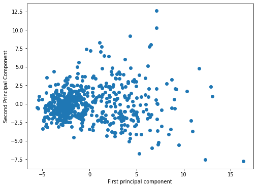

PLOT

from sklearn.datasets import load_breast_cancer

# REQUIRES INTERNET CONNECTION AND FIREWALL ACCESS
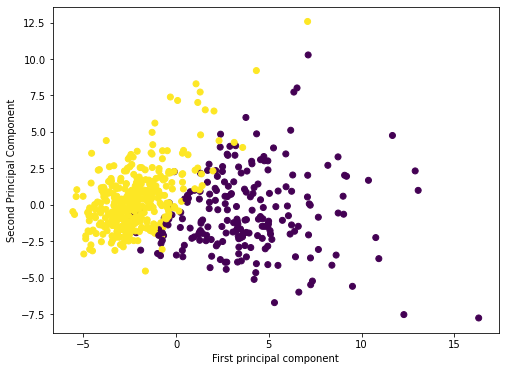
cancer_dictionary = load_breast_cancer()

cancer_dictionary.keys()

RESULT

dict_keys(['data', 'target', 'frame', 'target_names', 'DESCR', 'feature_names', 'filename'])

cancer_dictionary['target']

RESULT

array([0, 0, 0, 0, 0, 0, 0, 0, 0, 0, 0, 0, 0, 0, 0, 0, 0, 0, 0, 1, 1, 1,
       0, 0, 0, 0, 0, 0, 0, 0, 0, 0, 0, 0, 0, 0, 0, 1, 0, 0, 0, 0, 0, 0,
       0, 0, 1, 0, 1, 1, 1, 1, 1, 0, 0, 1, 0, 0, 1, 1, 1, 1, 0, 1, 0, 0,
       1, 1, 1, 1, 0, 1, 0, 0, 1, 0, 1, 0, 0, 1, 1, 1, 0, 0, 1, 0, 0, 0,
       1, 1, 1, 0, 1, 1, 0, 0, 1, 1, 1, 0, 0, 1, 1, 1, 1, 0, 1, 1, 0, 1,

plt.figure(figsize=(8,6))
plt.scatter(principal_components[:,0],principal_components[:,1],c=cancer_dictionary['target'])
plt.xlabel('First principal component')
plt.ylabel('Second Principal Component')

RESULT

Text(0, 0.5, 'Second Principal Component')

PLOT

DBSCAN 01 Pca Scikit Learn