++++

Data Science

May 2026×Notebook lesson

Notebook converted from Jupyter for blog publishing.

00-AdaBoost

Driptanil DattaSoftware Developer

AdaBoost

The Data

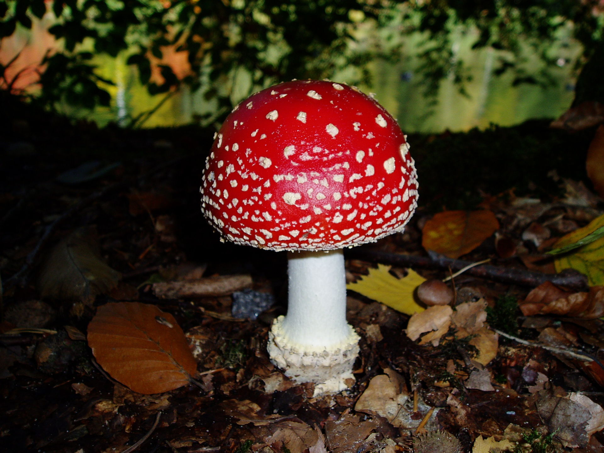
Mushroom Hunting: Edible or Poisonous?

Data Source: https://archive.ics.uci.edu/ml/datasets/Mushroom (opens in a new tab)

This data set includes descriptions of hypothetical samples corresponding to 23 species of gilled mushrooms in the Agaricus and Lepiota Family (pp. 500-525). Each species is identified as definitely edible, definitely poisonous, or of unknown edibility and not recommended. This latter class was combined with the poisonous one. The Guide clearly states that there is no simple rule for determining the edibility of a mushroom; no rule like ``leaflets three, let it be'' for Poisonous Oak and Ivy.

Attribute Information:

1. cap-shape: bell=b,conical=c,convex=x,flat=f, knobbed=k,sunken=s
2. cap-surface: fibrous=f,grooves=g,scaly=y,smooth=s
3. cap-color: brown=n,buff=b,cinnamon=c,gray=g,green=r, pink=p,purple=u,red=e,white=w,yellow=y
4. bruises?: bruises=t,no=f
5. odor: almond=a,anise=l,creosote=c,fishy=y,foul=f, musty=m,none=n,pungent=p,spicy=s
6. gill-attachment: attached=a,descending=d,free=f,notched=n
7. gill-spacing: close=c,crowded=w,distant=d
8. gill-size: broad=b,narrow=n
9. gill-color: black=k,brown=n,buff=b,chocolate=h,gray=g, green=r,orange=o,pink=p,purple=u,red=e, white=w,yellow=y
10. stalk-shape: enlarging=e,tapering=t
11. stalk-root: bulbous=b,club=c,cup=u,equal=e, rhizomorphs=z,rooted=r,missing=?
12. stalk-surface-above-ring: fibrous=f,scaly=y,silky=k,smooth=s
13. stalk-surface-below-ring: fibrous=f,scaly=y,silky=k,smooth=s
14. stalk-color-above-ring: brown=n,buff=b,cinnamon=c,gray=g,orange=o, pink=p,red=e,white=w,yellow=y
15. stalk-color-below-ring: brown=n,buff=b,cinnamon=c,gray=g,orange=o, pink=p,red=e,white=w,yellow=y
16. veil-type: partial=p,universal=u
17. veil-color: brown=n,orange=o,white=w,yellow=y
18. ring-number: none=n,one=o,two=t
19. ring-type: cobwebby=c,evanescent=e,flaring=f,large=l, none=n,pendant=p,sheathing=s,zone=z
20. spore-print-color: black=k,brown=n,buff=b,chocolate=h,green=r, orange=o,purple=u,white=w,yellow=y
21. population: abundant=a,clustered=c,numerous=n, scattered=s,several=v,solitary=y
22. habitat: grasses=g,leaves=l,meadows=m,paths=p, urban=u,waste=w,woods=d

Goal

THIS IS IMPORTANT, THIS IS NOT OUR TYPICAL PREDICTIVE MODEL!

Our general goal here is to see if we can harness the power of machine learning and boosting to help create not just a predictive model, but a general guideline for features people should look out for when picking mushrooms.

Imports

import numpy as np
import pandas as pd
 
import matplotlib.pyplot as plt
import seaborn as sns

df = pd.read_csv("../DATA/mushrooms.csv")

df.head()

class
cap-shape
cap-surface
cap-color
bruises

EDA

sns.countplot(data=df,x='class')

<AxesSubplot:xlabel='class', ylabel='count'>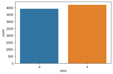

PLOT

df.describe()

class
cap-shape
cap-surface
cap-color
bruises

df.describe().transpose()

count
unique
top
freq
class

plt.figure(figsize=(14,6),dpi=200)
sns.barplot(data=df.describe().transpose().reset_index().sort_values('unique'),x='index',y='unique')
plt.xticks(rotation=90);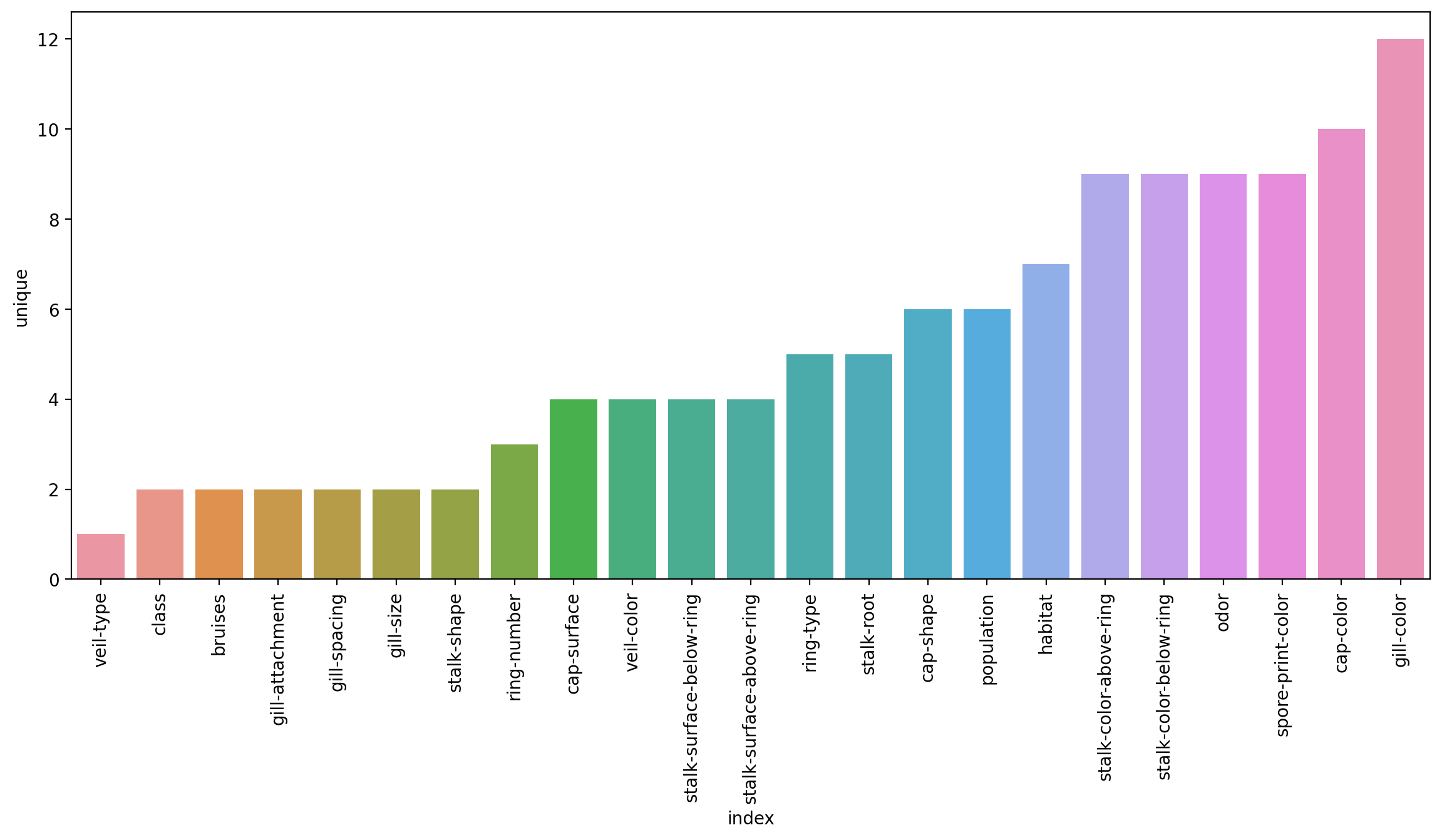

PLOT

Train Test Split

X = df.drop('class',axis=1)

X = pd.get_dummies(X,drop_first=True)

y = df['class']

from sklearn.model_selection import train_test_split

X_train, X_test, y_train, y_test = train_test_split(X, y, test_size=0.15, random_state=101)

Modeling

from sklearn.ensemble import AdaBoostClassifier

model = AdaBoostClassifier(n_estimators=1)

model.fit(X_train,y_train)

AdaBoostClassifier(n_estimators=1)

Evaluation

from sklearn.metrics import classification_report,plot_confusion_matrix,accuracy_score

predictions = model.predict(X_test)

predictions

array(['p', 'e', 'p', ..., 'p', 'p', 'e'], dtype=object)

print(classification_report(y_test,predictions))

              precision    recall  f1-score   support

           e       0.96      0.81      0.88       655
           p       0.81      0.96      0.88       564

model.feature_importances_

array([0., 0., 0., 0., 0., 0., 0., 0., 0., 0., 0., 0., 0., 0., 0., 0., 0.,
       0., 0., 0., 0., 0., 1., 0., 0., 0., 0., 0., 0., 0., 0., 0., 0., 0.,
       0., 0., 0., 0., 0., 0., 0., 0., 0., 0., 0., 0., 0., 0., 0., 0., 0.,
       0., 0., 0., 0., 0., 0., 0., 0., 0., 0., 0., 0., 0., 0., 0., 0., 0.,
       0., 0., 0., 0., 0., 0., 0., 0., 0., 0., 0., 0., 0., 0., 0., 0., 0.,

model.feature_importances_.argmax()

22

X.columns[22]

'odor_n'

sns.countplot(data=df,x='odor',hue='class')

<AxesSubplot:xlabel='odor', ylabel='count'>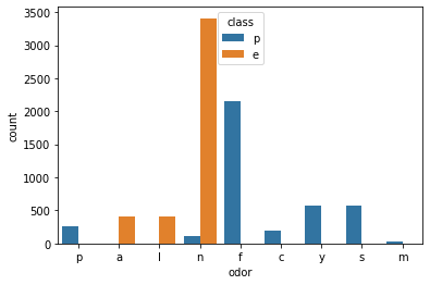

PLOT

Analyzing performance as more weak learners are added.

len(X.columns)

95

error_rates = []
 
for n in range(1,96):
    
    model = AdaBoostClassifier(n_estimators=n)
    model.fit(X_train,y_train)
    preds = model.predict(X_test)
    err = 1 - accuracy_score(y_test,preds)
    
    error_rates.append(err)

plt.plot(range(1,96),error_rates)

[<matplotlib.lines.Line2D at 0x289c33b1f70>]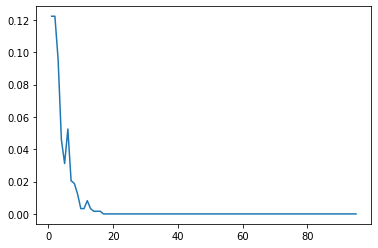

PLOT

model

AdaBoostClassifier(n_estimators=95)

model.feature_importances_

array([0.        , 0.        , 0.        , 0.        , 0.        ,
       0.        , 0.        , 0.        , 0.01052632, 0.        ,
       0.        , 0.01052632, 0.        , 0.        , 0.        ,
       0.01052632, 0.        , 0.05263158, 0.03157895, 0.03157895,
       0.        , 0.        , 0.06315789, 0.02105263, 0.        ,

feats = pd.DataFrame(index=X.columns,data=model.feature_importances_,columns=['Importance'])

feats

Importance
cap-shape_c
0.000000
cap-shape_f
0.000000

imp_feats = feats[feats['Importance']>0]

imp_feats

Importance
cap-color_c
0.010526
cap-color_n
0.010526

imp_feats = imp_feats.sort_values("Importance")

plt.figure(figsize=(14,6),dpi=200)
sns.barplot(data=imp_feats.sort_values('Importance'),x=imp_feats.sort_values('Importance').index,y='Importance')
 
plt.xticks(rotation=90);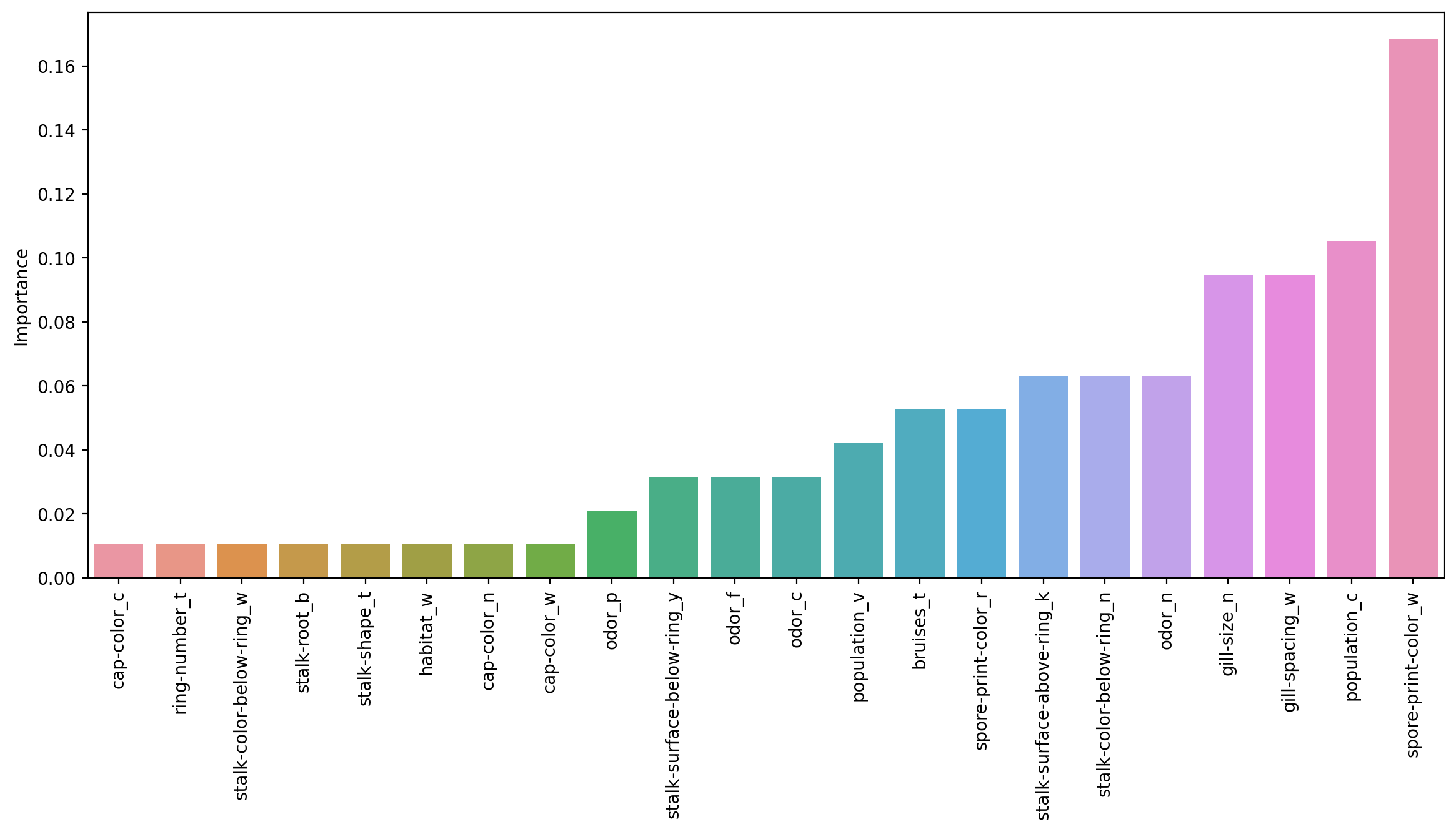

PLOT

sns.countplot(data=df,x='habitat',hue='class')

<AxesSubplot:xlabel='habitat', ylabel='count'>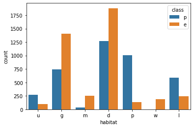

PLOT

Interesting to see how the importance of the features shift as more are allowed to be added in! But remember these are all weak learner stumps, and feature importance is available for all the tree methods!