++++

Data Science

May 2026×Notebook lesson

Notebook converted from Jupyter for blog publishing.

01-Random-Forest-Regression

Driptanil DattaSoftware Developer

Random Forest - Regression

Plus: An Additional Analysis of Various Regression Methods!

The Data

We just got hired by a tunnel boring company which uses X-rays in an attempt to know rock density, ideally this will allow them to switch out boring heads on their equipment before having to mine through the rock!

They have given us some lab test results of signal strength returned in nHz to their sensors for various rock density types tested. You will notice it has almost a sine wave like relationship, where signal strength oscillates based off the density, the researchers are unsure why this is, but

import numpy as np
import pandas as pd
import matplotlib.pyplot as plt
import seaborn as sns

df = pd.read_csv("../DATA/rock_density_xray.csv")

df.head()

HTML

Rebound Signal Strength nHz
Rock Density kg/m3
0
72.945124
2.456548

df.columns=['Signal',"Density"]

plt.figure(figsize=(12,8),dpi=200)
sns.scatterplot(x='Signal',y='Density',data=df)

RESULT

<AxesSubplot:xlabel='Signal', ylabel='Density'>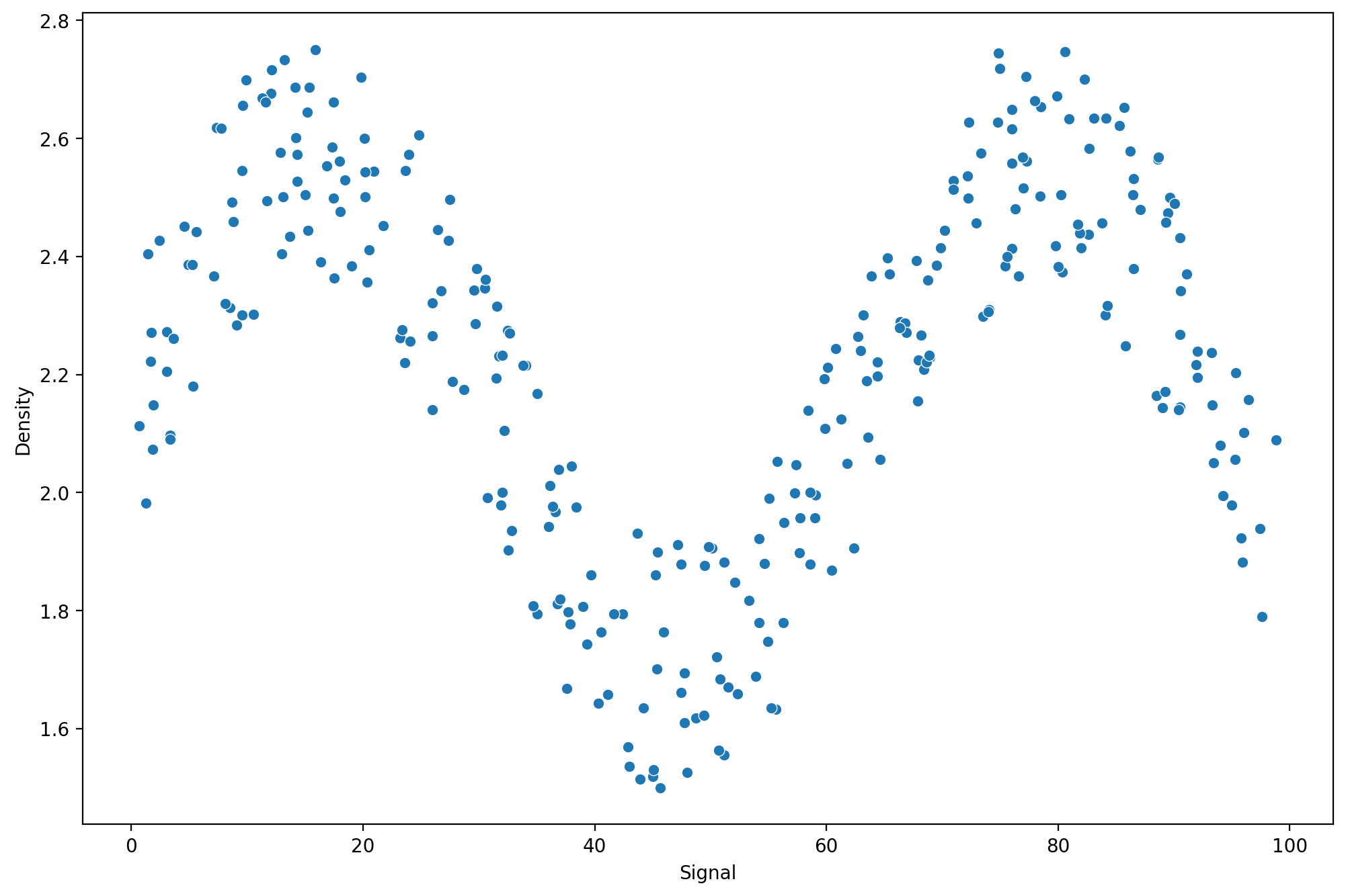

PLOT

Splitting the Data

Let's split the data in order to be able to have a Test set for performance metric evaluation.

X = df['Signal'].values.reshape(-1,1)  
y = df['Density']

from sklearn.model_selection import train_test_split

X_train, X_test, y_train, y_test = train_test_split(X, y, test_size=0.1, random_state=101)

Linear Regression

from sklearn.linear_model import LinearRegression

lr_model = LinearRegression()

lr_model.fit(X_train,y_train)

RESULT

LinearRegression()

lr_preds = lr_model.predict(X_test)

from sklearn.metrics import mean_squared_error

np.sqrt(mean_squared_error(y_test,lr_preds))

RESULT

0.2570051996584629

What does the fit look like?

signal_range = np.arange(0,100)

lr_output = lr_model.predict(signal_range.reshape(-1,1))

plt.figure(figsize=(12,8),dpi=200)
sns.scatterplot(x='Signal',y='Density',data=df,color='black')
plt.plot(signal_range,lr_output)

RESULT

[<matplotlib.lines.Line2D at 0x216f1c9c490>]

PLOT

Polynomial Regression

Attempting with a Polynomial Regression Model

Let's explore why our standard regression approach of a polynomial could be difficult to fit here, keep in mind, we're in a fortunate situation where we can easily visualize results of y vs x.

Function to Help Run Models

from sklearn.linear_model import LinearRegression
model = LinearRegression()

def run_model(model,X_train,y_train,X_test,y_test):
    
    # Fit Model
    model.fit(X_train,y_train)
    
    # Get Metrics
    
    preds = model.predict(X_test)
    
    rmse = np.sqrt(mean_squared_error(y_test,preds))
    print(f'RMSE : {rmse}')
    
    # Plot results
    signal_range = np.arange(0,100)
    output = model.predict(signal_range.reshape(-1,1))
    
    
    plt.figure(figsize=(12,6),dpi=150)
    sns.scatterplot(x='Signal',y='Density',data=df,color='black')
    plt.plot(signal_range,output)

run_model(model,X_train,y_train,X_test,y_test)

STDOUT

RMSE : 0.2570051996584629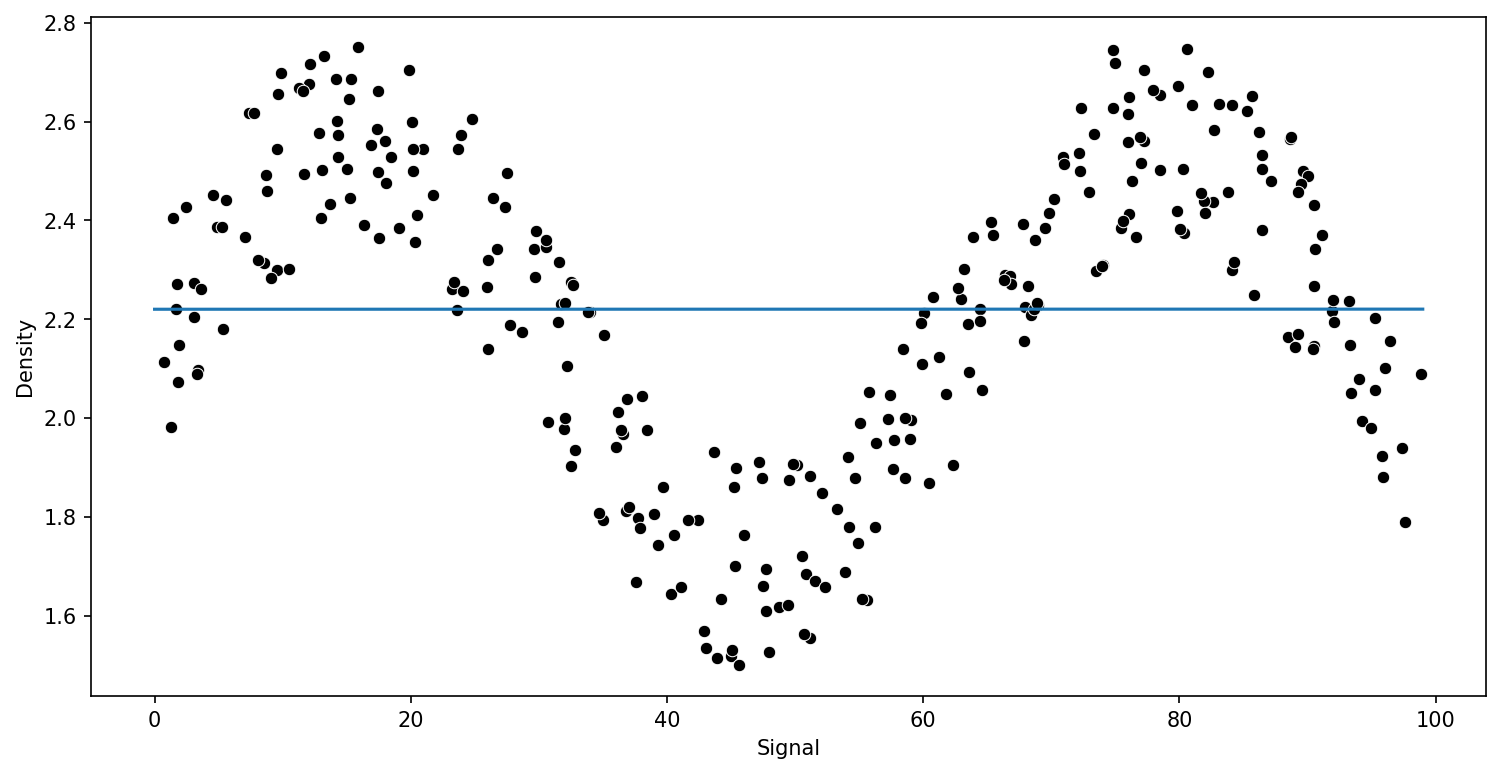

PLOT

Pipeline for Poly Orders

from sklearn.pipeline import make_pipeline

from sklearn.preprocessing import PolynomialFeatures

pipe = make_pipeline(PolynomialFeatures(2),LinearRegression())

run_model(pipe,X_train,y_train,X_test,y_test)

STDOUT

RMSE : 0.2817309563725596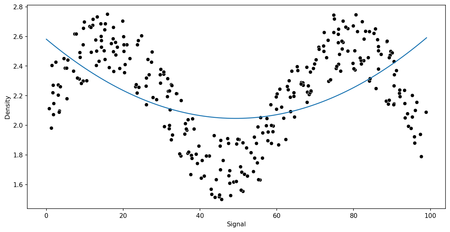

PLOT

Comparing Various Polynomial Orders

pipe = make_pipeline(PolynomialFeatures(10),LinearRegression())
run_model(pipe,X_train,y_train,X_test,y_test)

STDOUT

RMSE : 0.1417947898442399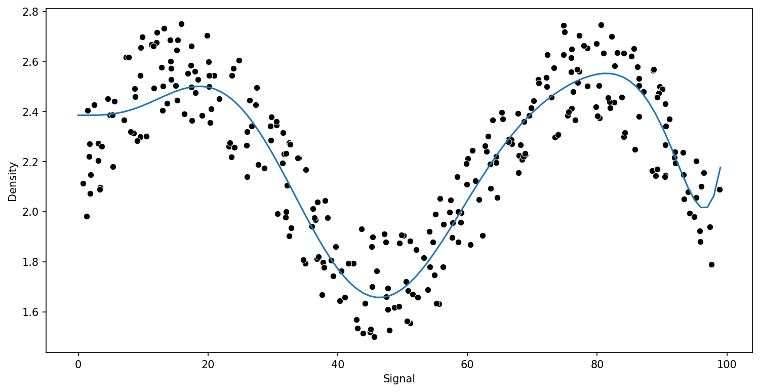

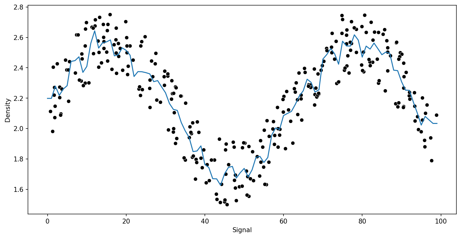
PLOT

KNN Regression

from sklearn.neighbors import KNeighborsRegressor

preds = {}
k_values = [1,5,10]
for n in k_values:
    
    
    model = KNeighborsRegressor(n_neighbors=n)
    run_model(model,X_train,y_train,X_test,y_test)

STDOUT

RMSE : 0.15234870286353372
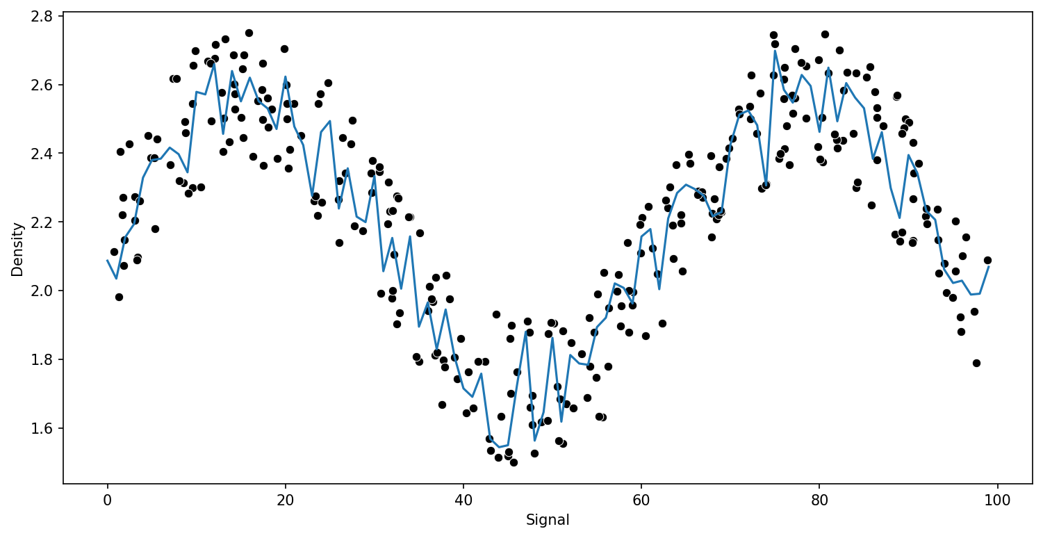
RMSE : 0.13730685016923655
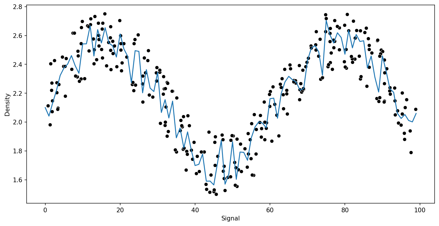
RMSE : 0.13277855732740926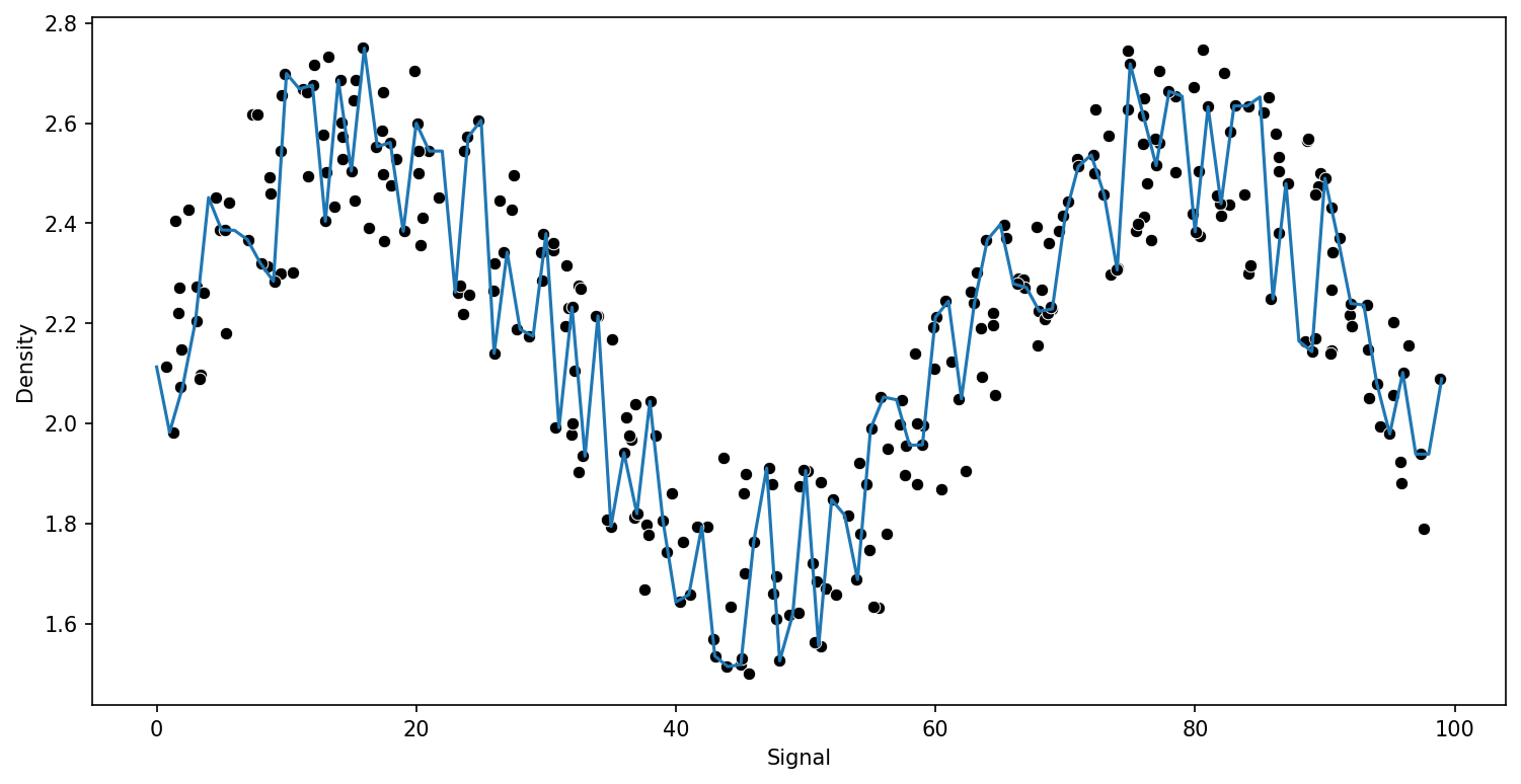

PLOT

PLOT

PLOT

Decision Tree Regression

from sklearn.tree import DecisionTreeRegressor

model = DecisionTreeRegressor()
 
run_model(model,X_train,y_train,X_test,y_test)

STDOUT

RMSE : 0.15234870286353372

PLOT

model.get_n_leaves()

RESULT

Support Vector Regression

from sklearn.svm import SVR

from sklearn.model_selection import GridSearchCV

param_grid = {'C':[0.01,0.1,1,5,10,100,1000],'gamma':['auto','scale']}
svr = SVR()

grid = GridSearchCV(svr,param_grid)

run_model(grid,X_train,y_train,X_test,y_test)

STDOUT

RMSE : 0.12634668775105407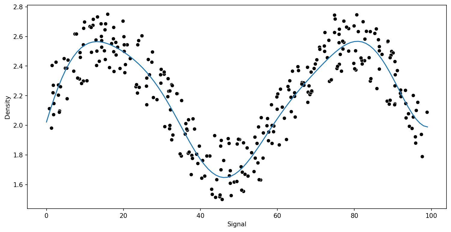

PLOT

grid.best_estimator_

RESULT

SVR(C=1000)

Random Forest Regression

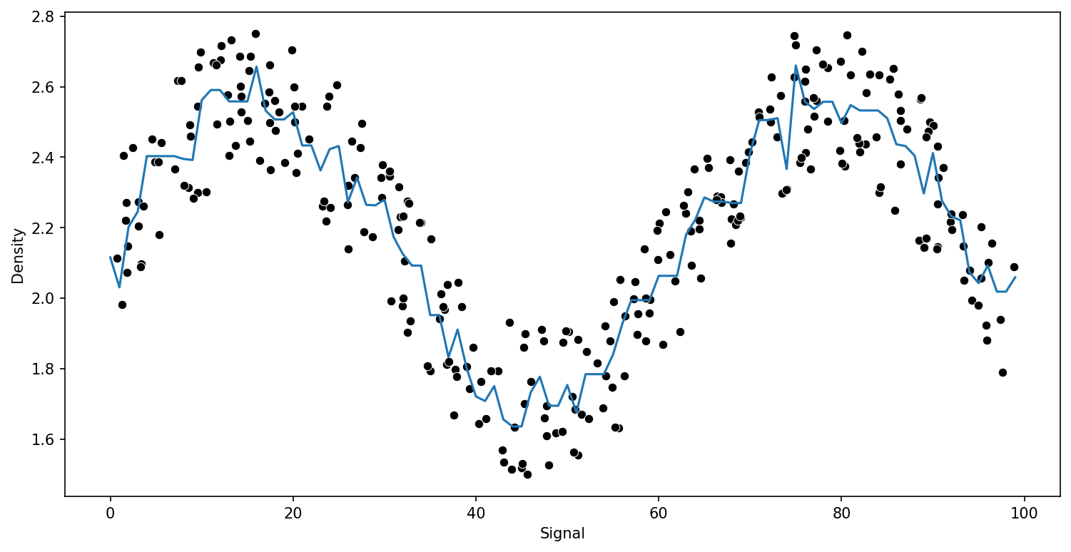
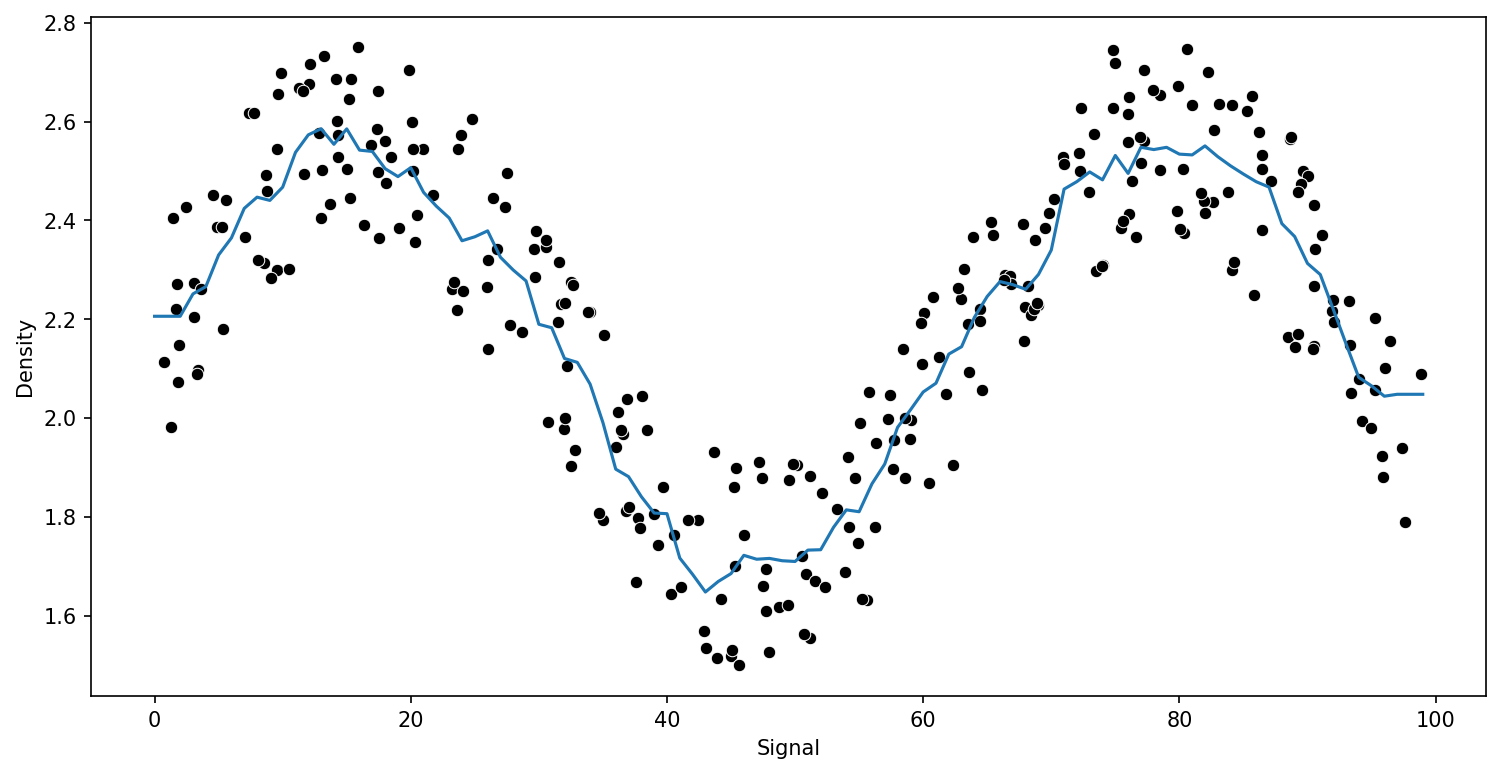
from sklearn.ensemble import RandomForestRegressor

# help(RandomForestRegressor)

trees = [10,50,100]
for n in trees:
    
    model = RandomForestRegressor(n_estimators=n)
    
    run_model(model,X_train,y_train,X_test,y_test)

STDOUT

RMSE : 0.1417613358931285
RMSE : 0.133281449397454
RMSE : 0.13699094997283662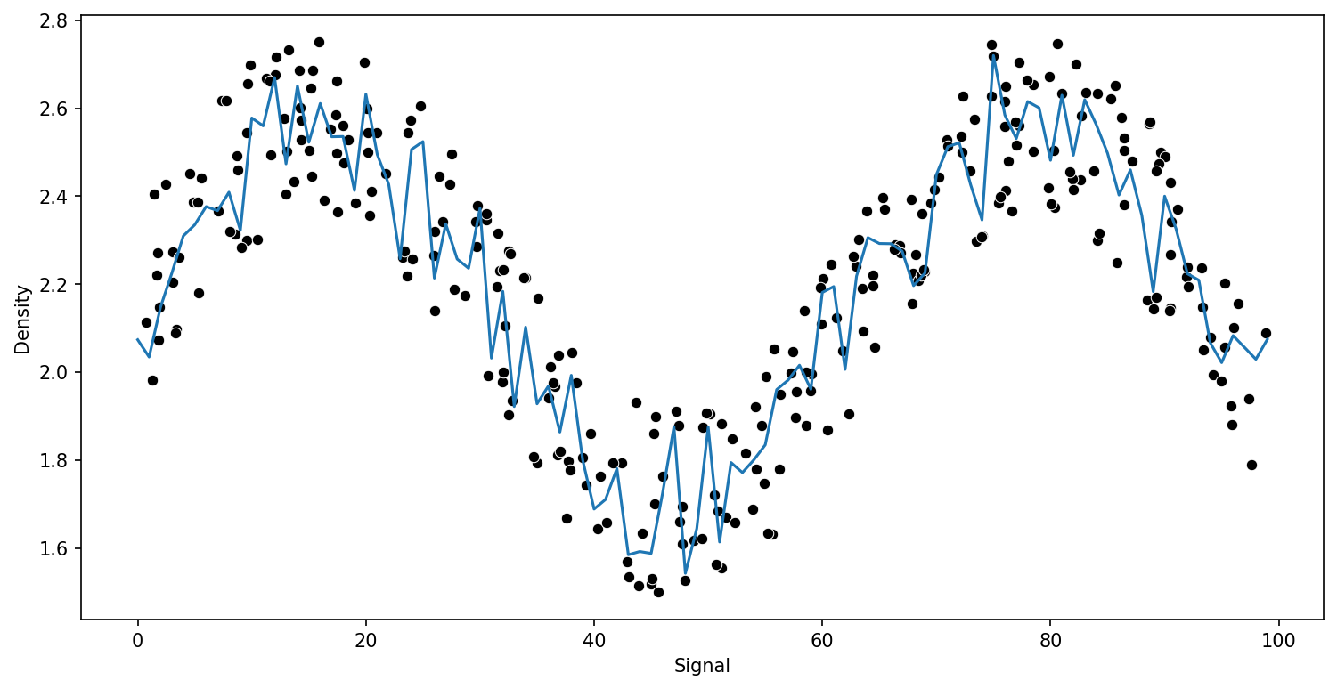

PLOT

PLOT

PLOT

Gradient Boosting

We will cover this in more detail in next section.

from sklearn.ensemble import GradientBoostingRegressor

# help(GradientBoostingRegressor)

   
model = GradientBoostingRegressor()
 
run_model(model,X_train,y_train,X_test,y_test)

STDOUT

RMSE : 0.13294148649584667

PLOT

Adaboost

from sklearn.ensemble import AdaBoostRegressor

model = GradientBoostingRegressor()
 
run_model(model,X_train,y_train,X_test,y_test)

STDOUT

RMSE : 0.13294148649584667

PLOT

00 Random Forest Classification Random Forests