++++

Data Science

May 2026×Notebook lesson

Notebook converted from Jupyter for blog publishing.

05-Linear-Regression-Execise

Driptanil DattaSoftware Developer

import numpy as np
import pandas as pd
import matplotlib.pyplot as plt
import seaborn as sns

df = pd.read_csv("Advertising.csv")

df.head()

HTML

TV
radio
newspaper
sales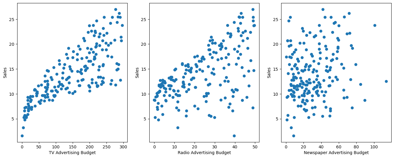
0

fig,axes = plt.subplots(nrows=1, ncols=3, figsize=(16,6))
 
axes[0].plot(df['TV'], df['sales'], 'o')
axes[0].set_ylabel('Sales')
axes[0].set_xlabel('TV Advertising Budget')
 
axes[1].plot(df['radio'], df['sales'], 'o')
axes[1].set_ylabel('Sales')
axes[1].set_xlabel('Radio Advertising Budget')
 
axes[2].plot(df['newspaper'], df['sales'], 'o')
axes[2].set_ylabel('Sales')
axes[2].set_xlabel('Newspaper Advertising Budget')

RESULT

Text(0.5, 0, 'Newspaper Advertising Budget')

PLOT

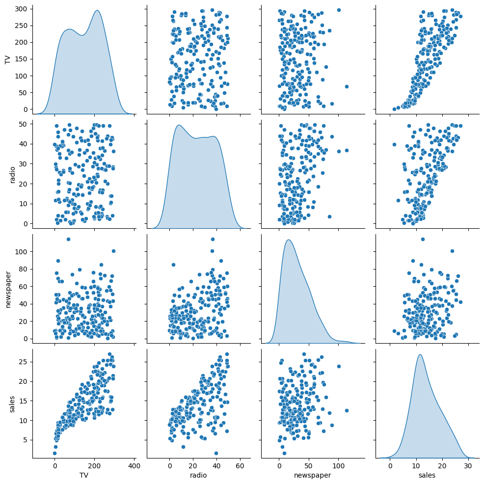
sns.pairplot(df, diag_kind='kde')

RESULT

<seaborn.axisgrid.PairGrid at 0x121816960>

PLOT

X = df.drop('sales', axis=1)
y = df['sales']

from sklearn.model_selection import train_test_split
 
X_train, X_test, y_train, y_test = train_test_split(X, y, test_size=0.2, random_state=42)

X_train

HTML

TV
radio
newspaper
79
116.0

y_train

RESULT

79     11.0
197    12.8
38     10.1
24      9.7
122    11.6

from sklearn.linear_model import LinearRegression

model = LinearRegression()
 
# Model Training on Data
model.fit(X_train, y_train)

HTML

LinearRegression()In a Jupyter environment, please rerun this cell to show the HTML representation or trust the notebook.
On GitHub, the HTML representation is unable to render, please try loading this page with nbviewer.org.
LinearRegression
?Documentation for LinearRegressioniFitted
Parameters

test_predictions = model.predict(X_test)

test_predictions

RESULT

array([16.4080242 , 20.88988209, 21.55384318, 10.60850256, 22.11237326,
       13.10559172, 21.05719192,  7.46101034, 13.60634581, 15.15506967,
        9.04831992,  6.65328312, 14.34554487,  8.90349333,  9.68959028,
       12.16494386,  8.73628397, 16.26507258, 10.27759582, 18.83109103,
       19.56036653, 13.25103464, 12.33620695, 21.30695132,  7.82740305,

from sklearn.metrics import mean_absolute_error,mean_squared_error

MAE = mean_absolute_error(y_test, test_predictions)
MSE = mean_squared_error(y_test, test_predictions)
RMSE = np.sqrt(MSE)

print(f"Mean Absolute Error: {MAE}")
print(f"Mean Squared Error: {MSE}")
print(f"Root Mean Squared Error: {RMSE}")

STDOUT

Mean Absolute Error: 1.4607567168117606
Mean Squared Error: 3.174097353976105
Root Mean Squared Error: 1.7815996615334504

df['sales'].mean()

RESULT

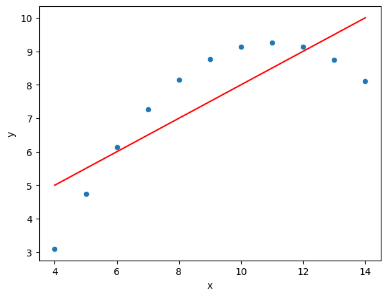
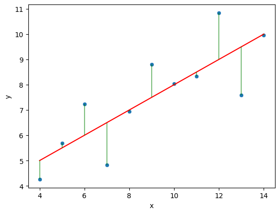
np.float64(14.0225)

quartet = pd.read_csv('anscombes_quartet1.csv')

quartet['pred_y'] = 3 + 0.5 * quartet['x']
quartet['residual'] = quartet['y'] - quartet['pred_y']
 
sns.scatterplot(data=quartet, x='x', y='y')
sns.lineplot(data=quartet, x='x', y='pred_y', color='red')
plt.vlines(x=quartet['x'], ymin=quartet['pred_y'], ymax=quartet['y'], color='green', alpha=0.5)

RESULT

<matplotlib.collections.LineCollection at 0x1245f70b0>

PLOT

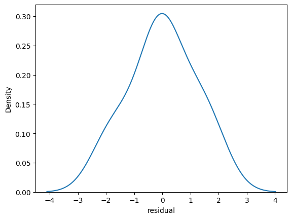
sns.kdeplot(quartet['residual'])

RESULT

<Axes: xlabel='residual', ylabel='Density'>

PLOT

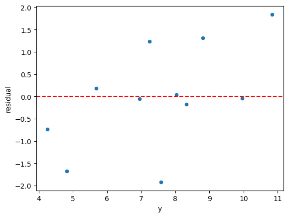
sns.scatterplot(data=quartet,x='y',y='residual')
plt.axhline(y=0, color='r', linestyle='--')

RESULT

<matplotlib.lines.Line2D at 0x124730d40>

PLOT

quartet = pd.read_csv('anscombes_quartet2.csv')

quartet.columns = ['x','y']

# y = 3.00 + 0.500x
quartet['pred_y'] = 3 + 0.5 * quartet['x']
quartet['residual'] = quartet['y'] - quartet['pred_y']
 
sns.scatterplot(data=quartet,x='x',y='y')
sns.lineplot(data=quartet,x='x',y='pred_y',color='red')
plt.vlines(quartet['x'],quartet['y'],quartet['y']-quartet['residual'])

RESULT

<Axes: xlabel='x', ylabel='y'>

PLOT

04 Linear Regression Project Dataset Linear Regression Models