++++

Data Science

May 2026×Notebook lesson

Notebook converted from Jupyter for blog publishing.

02-Polynomial-Regression

Driptanil DattaSoftware Developer

Polynomial Regression with SciKit-Learn

We saw how to create a very simple best fit line, but now let's greatly expand our toolkit to start thinking about the considerations of overfitting, underfitting, model evaluation, as well as multiple features!

Imports

import numpy as np
import pandas as pd
import matplotlib.pyplot as plt
import seaborn as sns

Sample Data

This sample data is from ISLR. It displays sales (in thousands of units) for a particular product as a function of advertising budgets (in thousands of dollars) for TV, radio, and newspaper media.

df = pd.read_csv("Advertising.csv")

df.head()

TV
radio
newspaper
sales
0

# Everything BUT the sales column
X = df.drop('sales',axis=1)

y = df['sales']

SciKit Learn

Polynomial Regression

From Preprocessing, import PolynomialFeatures, which will help us transform our original data set by adding polynomial features

We will go from the equation in the form (shown here as if we only had one x feature):

$\hat{y} = \beta_0 + \beta_1x_1 + \epsilon$

and create more features from the original x feature for some d degree of polynomial.

$\hat{y} = \beta_0 + \beta_1x_1 + \beta_1x^2_1 + ... + \beta_dx^d_1 + \epsilon$

Then we can call the linear regression model on it, since in reality, we're just treating these new polynomial features x^2, x^3, ... x^d as new features. Obviously we need to be careful about choosing the correct value of d , the degree of the model. Our metric results on the test set will help us with this!

The other thing to note here is we have multiple X features, not just a single one as in the formula above, so in reality, the PolynomialFeatures will also take interaction terms into account for example, if an input sample is two dimensional and of the form [a, b], the degree-2 polynomial features are [1, a, b, a^2, ab, b^2].

from sklearn.preprocessing import PolynomialFeatures

polynomial_converter = PolynomialFeatures(degree=2,include_bias=False)

# Converter "fits" to data, in this case, reads in every X column
# Then it "transforms" and ouputs the new polynomial data
poly_features = polynomial_converter.fit_transform(X)

poly_features.shape

(200, 9)

X.shape

(200, 3)

X.iloc[0]

TV           230.1
radio         37.8
newspaper     69.2
Name: 0, dtype: float64

poly_features[0]

array([2.301000e+02, 3.780000e+01, 6.920000e+01, 5.294601e+04,
       8.697780e+03, 1.592292e+04, 1.428840e+03, 2.615760e+03,
       4.788640e+03])

poly_features[0][:3]

array([230.1,  37.8,  69.2])

poly_features[0][:3]**2

array([52946.01,  1428.84,  4788.64])

The interaction terms $x_1 \cdot x_2 \text{ and } x_1 \cdot x_3 \text{ and } x_2 \cdot x_3$

230.1*37.8

8697.779999999999

230.1*69.2

15922.92

37.8*69.2

2615.7599999999998

Train | Test Split

Make sure you have watched the Machine Learning Overview videos on Supervised Learning to understand why we do this step

from sklearn.model_selection import train_test_split

# random_state: 
# https://stackoverflow.com/questions/28064634/random-state-pseudo-random-number-in-scikit-learn
X_train, X_test, y_train, y_test = train_test_split(poly_features, y, test_size=0.3, random_state=101)

Model for fitting on Polynomial Data

Create an instance of the model with parameters

from sklearn.linear_model import LinearRegression

model = LinearRegression(fit_intercept=True)

Fit/Train the Model on the training data

Make sure you only fit to the training data, in order to fairly evaluate your model's performance on future data

model.fit(X_train,y_train)

LinearRegression(copy_X=True, fit_intercept=True, n_jobs=None, normalize=False)

Evaluation on the Test Set

Calculate Performance on Test Set

We want to fairly evaluate our model, so we get performance metrics on the test set (data the model has never seen before).

test_predictions = model.predict(X_test)

from sklearn.metrics import mean_absolute_error,mean_squared_error

MAE = mean_absolute_error(y_test,test_predictions)
MSE = mean_squared_error(y_test,test_predictions)
RMSE = np.sqrt(MSE)

MAE

0.489679804480361

MSE

0.4417505510403426

RMSE

0.6646431757269028

df['sales'].mean()

14.022500000000003

Comparison with Simple Linear Regression

Results on the Test Set (Note: Use the same Random Split to fairly compare!)

• Simple Linear Regression:

  • MAE: 1.213
  • RMSE: 1.516

• Polynomial 2-degree:

  • MAE: 0.4896
  • RMSE: 0.664

Choosing a Model

Adjusting Parameters

Are we satisfied with this performance? Perhaps a higher order would improve performance even more! But how high is too high? It is now up to us to possibly go back and adjust our model and parameters, let's explore higher order Polynomials in a loop and plot out their error. This will nicely lead us into a discussion on Overfitting.

Let's use a for loop to do the following:

1. Create different order polynomial X data
2. Split that polynomial data for train/test
3. Fit on the training data
4. Report back the metrics on both the train and test results
5. Plot these results and explore overfitting

# TRAINING ERROR PER DEGREE
train_rmse_errors = []
# TEST ERROR PER DEGREE
test_rmse_errors = []
 
for d in range(1,10):
    
    # CREATE POLY DATA SET FOR DEGREE "d"
    polynomial_converter = PolynomialFeatures(degree=d,include_bias=False)
    poly_features = polynomial_converter.fit_transform(X)
    
    # SPLIT THIS NEW POLY DATA SET
    X_train, X_test, y_train, y_test = train_test_split(poly_features, y, test_size=0.3, random_state=101)
    
    # TRAIN ON THIS NEW POLY SET
    model = LinearRegression(fit_intercept=True)
    model.fit(X_train,y_train)
    
    # PREDICT ON BOTH TRAIN AND TEST
    train_pred = model.predict(X_train)
    test_pred = model.predict(X_test)
    
    # Calculate Errors
    
    # Errors on Train Set
    train_RMSE = np.sqrt(mean_squared_error(y_train,train_pred))
    
    # Errors on Test Set
    test_RMSE = np.sqrt(mean_squared_error(y_test,test_pred))
 
    # Append errors to lists for plotting later
    
   
    train_rmse_errors.append(train_RMSE)
    test_rmse_errors.append(test_RMSE)

plt.plot(range(1,6),train_rmse_errors[:5],label='TRAIN')
plt.plot(range(1,6),test_rmse_errors[:5],label='TEST')
plt.xlabel("Polynomial Complexity")
plt.ylabel("RMSE")
plt.legend()

<matplotlib.legend.Legend at 0x168c0d109c8>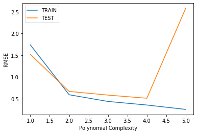

PLOT

plt.plot(range(1,10),train_rmse_errors,label='TRAIN')
plt.plot(range(1,10),test_rmse_errors,label='TEST')
plt.xlabel("Polynomial Complexity")
plt.ylabel("RMSE")
plt.legend()

<matplotlib.legend.Legend at 0x168c1d7df08>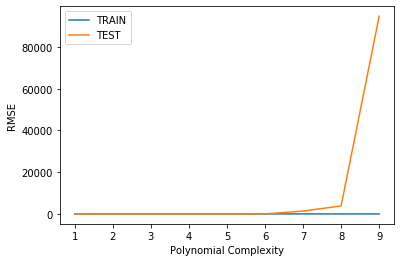

PLOT

plt.plot(range(1,10),train_rmse_errors,label='TRAIN')
plt.plot(range(1,10),test_rmse_errors,label='TEST')
plt.xlabel("Polynomial Complexity")
plt.ylabel("RMSE")
plt.ylim(0,100)
plt.legend()

<matplotlib.legend.Legend at 0x168c41e5a88>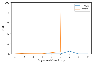

PLOT

Finalizing Model Choice

There are now 2 things we need to save, the Polynomial Feature creator AND the model itself. Let's explore how we would proceed from here:

1. Choose final parameters based on test metrics
2. Retrain on all data
3. Save Polynomial Converter object
4. Save model

# Based on our chart, could have also been degree=4, but 
# it is better to be on the safe side of complexity
final_poly_converter = PolynomialFeatures(degree=3,include_bias=False)

final_model = LinearRegression()

final_model.fit(final_poly_converter.fit_transform(X),y)

LinearRegression(copy_X=True, fit_intercept=True, n_jobs=None, normalize=False)

Saving Model and Converter

from joblib import dump, load

dump(final_model, 'sales_poly_model.joblib')

['sales_poly_model.joblib']

dump(final_poly_converter,'poly_converter.joblib')

['poly_converter.joblib']

Deployment and Predictions

Prediction on New Data

Recall that we will need to convert any incoming data to polynomial data, since that is what our model is trained on. We simply load up our saved converter object and only call .transform() on the new data, since we're not refitting to a new data set.

Our next ad campaign will have a total spend of 149k on TV, 22k on Radio, and 12k on Newspaper Ads, how many units could we expect to sell as a result of this?

loaded_poly = load('poly_converter.joblib')
loaded_model = load('sales_poly_model.joblib')

campaign = [[149,22,12]]

campaign_poly = loaded_poly.transform(campaign)

campaign_poly

array([[1.490000e+02, 2.200000e+01, 1.200000e+01, 2.220100e+04,
        3.278000e+03, 1.788000e+03, 4.840000e+02, 2.640000e+02,
        1.440000e+02, 3.307949e+06, 4.884220e+05, 2.664120e+05,
        7.211600e+04, 3.933600e+04, 2.145600e+04, 1.064800e+04,
        5.808000e+03, 3.168000e+03, 1.728000e+03]])

final_model.predict(campaign_poly)

array([14.64501014])