Adapted from A deep understanding of AI language model mechanisms — https://udemy.com/course/dullms_x
1. Setup and Environment
We'll start by importing our standard data science tools and configuring the plotting backend for high-quality SVG outputs.
import numpy as np
import matplotlib.pyplot as plt

import matplotlib_inline.backend_inline
matplotlib_inline.backend_inline.set_matplotlib_formats('svg')
2. Extracting Position Embeddings
We'll load the GPT-2 model and isolate the word position embedding (WPE) matrix to explore its internal correlations.
from transformers import GPT2Model

# get the Word Position Embeddings matrix
gpt2 = GPT2Model.from_pretrained('gpt2')
positions = gpt2.wpe.weight.detach().numpy()/Users/drippy/.pyenv/versions/3.12.6/lib/python3.12/site-packages/tqdm/auto.py:21: TqdmWarning: IProgress not found. Please update jupyter and ipywidgets. See https://ipywidgets.readthedocs.io/en/stable/user_install.html
from .autonotebook import tqdm as notebook_tqdm3. Cosine Similarity Distributions
We'll calculate the cosine similarity between token positions and across embedding dimensions to see how "time" and "features" are related.
# copied from "embed_positionEmbeddings.ipynb"

# cosine similarities for "time series" (token index)
Pnorm1 = positions / np.linalg.norm(positions,axis=1,keepdims=True)
cossim_tokens = Pnorm1 @ Pnorm1.T

# cosine similarities across embedding dimensions
Pnorm0 = positions / np.linalg.norm(positions,axis=0,keepdims=True)
cossim_embeds = Pnorm0.T @ Pnorm0
Visualizing Similarity Matrices
Plotting the similarity matrices helps us identify local clusters where nearby positions share similar embedding patterns.
# draw the images (also copied from previous code file)
fig,axs = plt.subplots(1,2,figsize=(12,5))

h = axs[0].imshow(cossim_tokens,vmin=-1,vmax=1)
axs[0].set(xlabel='Token index ("time")',ylabel='Token index ("time")',title='$S_c$ over "time"')
ch = fig.colorbar(h,ax=axs[0],pad=.02,fraction=.046)
ch.ax.tick_params(labelsize=10)
ch.ax.set_yticks(np.arange(-1,1.1,.5))

h = axs[1].imshow(cossim_embeds,vmin=-1,vmax=1)
axs[1].set(xlabel='Embedding index',ylabel='Embedding index',title='$S_c$ across embeddings')
ch = fig.colorbar(h,ax=axs[1],pad=.02,fraction=.046)
ch.ax.tick_params(labelsize=10)
ch.ax.set_yticks(np.arange(-1,1.1,.5))

plt.tight_layout()
plt.show()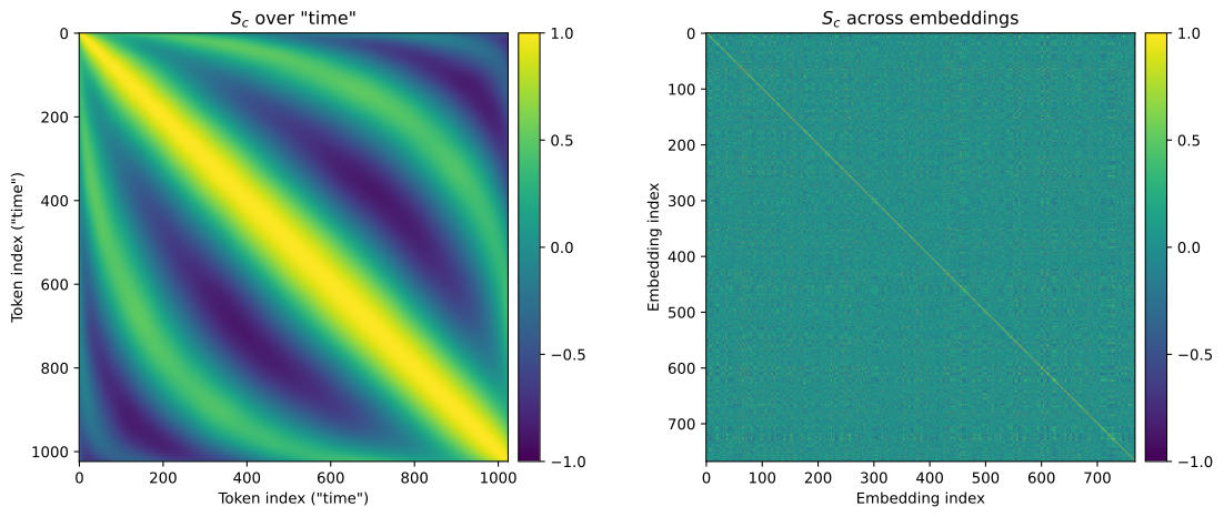
This reproduces the exact two heatmaps from the previous lesson: the temporal correlation ( over "time") on the left, and the feature correlation ( across embeddings) on the right.
Our goal now is to analyze the distribution of these similarities by plotting them as histograms. However, before we can feed this matrix data into a histogram, we must resolve two key mathematical redundancies:
- Symmetric redundancy: Cosine similarity is a symmetric measure of association. The similarity between token index $200$ and $600$ is identical to the similarity between index $600$ and $200$. Therefore, every pair similarity exists twice in the matrix (in the upper-right and lower-left halves).
- Trivial diagonal: The diagonal of the matrix represents the similarity of each vector with itself, which is trivially always $1.0$. This would create a massive artificial spike at the far-right edge of the histogram.
To address these issues, we can isolate only the unique, non-trivial elements using NumPy:
# small demo about triu:
A = np.random.randint(0,9,(4,4))
print(A)
print('')
A[np.nonzero(np.triu(A,1))][[7 2 1 7]
[5 8 7 8]
[4 1 8 4]
[4 3 3 0]]array([2, 1, 7, 7, 8, 4])Upper Triangle Extraction
To analyze the distribution of similarities without redundant diagonal values, we extract the unique upper-triangle elements.
# get the unique cosine similarity values from the upper-triangle
unique_cs_embeds = cossim_embeds[np.nonzero(np.triu(cossim_embeds,1))] # note the ",1" to avoid the trivial diagonal
unique_cs_tokens = cossim_tokens[np.nonzero(np.triu(cossim_tokens,1))]

# get their distributions
embed_hy,embed_hx = np.histogram(unique_cs_embeds,100)
token_hy,token_hx = np.histogram(unique_cs_tokens,100)

# visualize!
plt.figure(figsize=(12,4))
plt.bar(embed_hx[:-1],embed_hy,width=np.diff(embed_hx[:2]),alpha=.4,label='$S_c$ across embeddings')
plt.bar(token_hx[:-1],token_hy,width=np.diff(token_hx[:2]),alpha=.4,label='$S_c$ across "time"')
plt.plot(embed_hx[:-1],embed_hy)
plt.plot(token_hx[:-1],token_hy)

plt.legend()
plt.gca().set(xlim=[-1,1],xlabel='Cosine similarity',ylabel='Count',title='Distributions of $S_c$ in the positional embeddings matrix')
plt.show()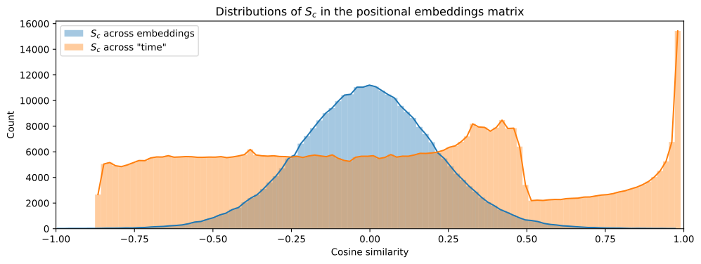
How We Isolated the Unique Associations
As introduced above, to avoid duplicating symmetric pairs and capturing the trivial diagonal values ($1.0$), we successfully isolated the upper triangle elements using our NumPy pipeline:
np.triu(cossim, k=1): Created the upper-triangular matrix, filtering out the diagonal and the lower-left symmetric values.np.nonzero(): Selected only the non-zero cells to build a clean 1D array of unique pairwise similarities.
Interpreting the Histogram Distributions
The resulting plot reveals the stark structural difference between the two similarity domains:
- Cosine Similarity Over "Time" (Orange): This distribution represents the unique token-index similarities. You'll notice it is much wider and distributed more broadly across the spectrum, reflecting the distinct structural patterns (the yellow and blue diagonal waves) learned by the model.
- Cosine Similarity Across Embeddings (Blue): This distribution represents the similarities between different embedding channels. It is highly concentrated, showing that most embedding dimensions have a narrow, specific similarity profile.
4. Shuffled Baseline Comparison
Is the structure we see in the position embeddings meaningful? We can test this by creating a shuffled version of the matrix and comparing its similarity distribution.
# vectorize and copy the positions
randomEmbeds = positions.flatten()

# randomly shuffle them
np.random.shuffle(randomEmbeds)

# reshape back to the matrix
randomEmbeds = randomEmbeds.reshape(positions.shape)
Shuffled Matrix Visualization
Visually comparing the real position matrix with the shuffled one reveals the systematic patterns that the model has learned during training.
_,axs = plt.subplots(2,1,figsize=(8,7))

axs[0].imshow(positions.T,aspect='auto',vmin=-.1,vmax=.1)
axs[0].set(xlabel='Token position',ylabel='Dimensions',title='GPT-2 position embeddings matrix')

axs[1].imshow(randomEmbeds.T,aspect='auto',vmin=-.1,vmax=.1)
axs[1].set(xlabel='Token position',ylabel='Dimensions',title='Shuffled embeddings matrix')


plt.tight_layout()
plt.show()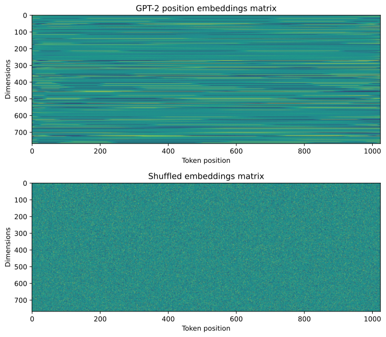
Calculating Shuffled Similarities
We'll compute the similarity distribution for the shuffled matrix to see how random noise compares to the model's learned structure.
# calculate cosine similarity
Rnorm0 = randomEmbeds / np.linalg.norm(randomEmbeds,axis=0,keepdims=True)
cossim_random = Rnorm0.T @ Rnorm0# get the unique cosine similarity values from the upper-triangle
unique_cs_random = cossim_random[np.nonzero(np.triu(cossim_random,1))]
# get their distribution
random_hy,random_hx = np.histogram(unique_cs_random,100)
# visualize!
plt.figure(figsize=(12,4))
plt.bar(embed_hx[:-1],embed_hy,width=np.diff(embed_hx[:2]),alpha=.4,label='$S_c$ across embeddings')
plt.bar(random_hx[:-1],random_hy,width=np.diff(random_hx[:2]),alpha=.4,label='$S_c$ in shuffled vectors')
plt.plot(embed_hx[:-1],embed_hy)
plt.plot(random_hx[:-1],random_hy)
plt.legend()
plt.gca().set(xlim=[-1,1],xlabel='Cosine similarity',ylabel='Count',title='Distributions of $S_c$ in the positional embeddings matrix')
plt.show()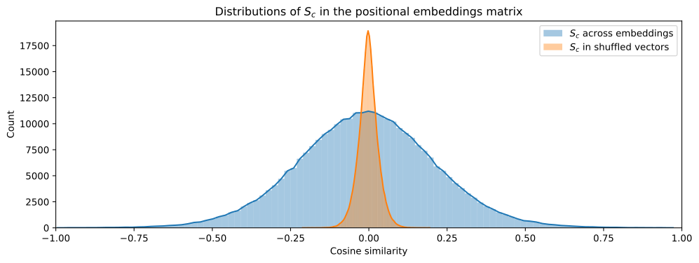
5. Identifying Highly Correlated Pairs
Finally, we'll identify the pairs of embedding dimensions that show the highest correlation and plot them against each other to visualize their relationship.
# reminder: positions matrix is size [index,embedding]

sortidx = np.argsort(np.triu(cossim_embeds,1).flatten())[::-1]
xx,yy = np.unravel_index(sortidx,cossim_embeds.shape)

for i in np.linspace(0,200,10).astype(int):

  # get and print the pairs
  pairname = f'({xx[i]},{yy[i]})'
  print(f'Cossim of {cossim_embeds[xx[i],yy[i]]:.3f} in pair {pairname}')

  # plot them
  plt.plot(positions[:,xx[i]],positions[:,yy[i]],'.-',alpha=.5,label=pairname)

# adjustments
plt.gca().set(xlabel='Embedding dimension "x"',ylabel='Embedding dimension "y"')
plt.legend(fontsize=9)
plt.show()Cossim of 0.992 in pair (356,528)
Cossim of 0.943 in pair (320,540)
Cossim of 0.915 in pair (308,528)
Cossim of 0.885 in pair (107,271)
Cossim of 0.864 in pair (365,525)5 more lines
Cossim of 0.845 in pair (479,623)
Cossim of 0.829 in pair (49,724)
Cossim of 0.813 in pair (71,365)
Cossim of 0.800 in pair (167,439)
Cossim of 0.794 in pair (527,623)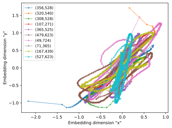
Key Take-home Points
- Structured Patterns: Learned position embeddings are not random noise; they exhibit clear semantic structures across both time and embedding dimensions.
- Temporal Localism: Nearby token positions show higher cosine similarity, confirming that the model learns a sense of local temporal context.
- Dimension Correlation: Certain embedding dimensions are highly correlated, suggesting that the model uses redundant features to represent position.
- Statistical Baseline: Shuffling the weights destroys these learned structures, resulting in a much narrower and centered similarity distribution.