Adapted from A deep understanding of AI language model mechanisms — https://udemy.com/course/dullms_x
1. Setup and Libraries
We'll start by importing our essential data science tools, including numpy for calculations, matplotlib for plotting, and sklearn and torch for built-in similarity metrics.
import numpy as np
import matplotlib.pyplot as plt

from sklearn.metrics.pairwise import cosine_similarity
import torch

# vector plots
import matplotlib_inline.backend_inline
matplotlib_inline.backend_inline.set_matplotlib_formats('svg')
2. Generating Sample Data
We'll generate three random datasets with varying degrees of correlation to demonstrate how cosine similarity behaves with different types of linear relationships.
# sample size
N = 30

# data vectors
d1 = np.random.randn(N) + 1 # add an offset for Pearson vs. cosine-similarity
d2 = d1 + np.random.randn(N)
d3 = -d1 + np.random.randn(N)

# visualize
_,axs = plt.subplots(1,3,figsize=(12,3.5))
axs[0].plot(d1,d2,'ks',markerfacecolor=[.7,.7,.9])
axs[0].set(xlabel='Data d1',ylabel='Data d2')

axs[1].plot(d1,d3,'ks',markerfacecolor=[.7,.9,.7])
axs[1].set(xlabel='Data d1',ylabel='Data d3')

axs[2].plot(d2,d3,'ks',markerfacecolor=[.9,.7,.7])
axs[2].set(xlabel='Data d2',ylabel='Data d3')

for a in axs: a.grid(linestyle='--',linewidth=.5)

plt.tight_layout()
plt.show()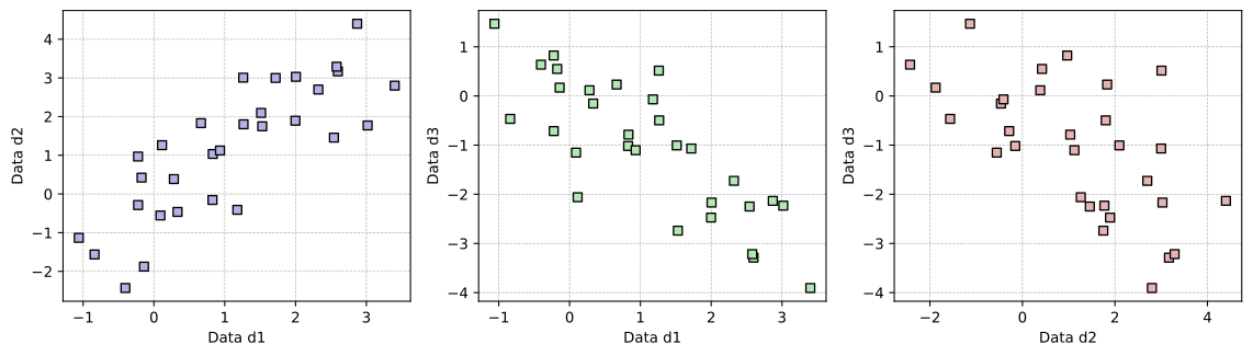
3. Manual Cosine Similarity Calculation
Before using library functions, it's helpful to implement the cosine similarity formula manually. It is calculated as the dot product of the vectors divided by the product of their magnitudes (Euclidean norms):
Where:
- Numerator: The dot product of the vectors.
- Denominator: The product of the Euclidean norms (L2 norms) of each vector.
Implementing this in Python:
# cosine similarity manual
num = sum( d1*d2 )
den = sum( d1*d1 ) * sum(d2**2)
cossim_manual = num/np.sqrt(den)

print(f'Manual calculation: Cosine similarity between d1 and d2 is {cossim_manual:.4f}')Manual calculation: Cosine similarity between d1 and d2 is 0.8769Verification with Sklearn
We can verify our manual calculation using the cosine_similarity function from scikit-learn.
Scikit-learn's pairwise metrics expect 2D arrays (samples features). Sinced1andd2are 1D vectors, we must use.reshape(1, -1)to convert them into 2D row vectors.
# check against sklearn
cossim_sklearn = cosine_similarity(d1.reshape(1, -1), d2.reshape(1, -1))
print(f'Sci-kit learn: Cosine similarity between d1 and d2 is {cossim_sklearn[0][0]:.4f}')Sci-kit learn: Cosine similarity between d1 and d2 is 0.8769print(d1.reshape(1,-1).shape)
print(d1.shape)(1, 30)
(30,)4. Relationship with Pearson Correlation
Cosine similarity and Pearson correlation are closely related. Specifically, cosine similarity on mean-centered data is mathematically equivalent to the Pearson correlation coefficient ().
By subtracting the mean () from the data, Pearson correlation removes any offset, focusing purely on the linear relationship between the variables.
# mean-center
d1m = d1 - np.mean(d1)
d2m = d2 - np.mean(d2)

# manual calculation
num = sum( d1m*d2m )
den = sum( d1m*d1m ) * sum( d2m*d2m )
corr_manual = num/np.sqrt(den)

# numpy
corr_np = np.corrcoef(d1,d2)[0,1]

# cosine similarity using mean-centered data
cossimM_sklearn = cosine_similarity(d1m.reshape(1,-1),d2m.reshape(1,-1))

# print all the results
print(f'Manual calculation: Pearson correlation between d1 and d2 is {corr_manual:.7f}')
print(f'Numpy corrcoef():   Pearson correlation between d1 and d2 is {corr_np:.7f}')
print(f'Sci-kit learn:      Cosine similarity between d1m and d2m is {cossimM_sklearn[0][0]:.7f}')
print(f'Sci-kit learn: Cosine similarity between d1 and d2 is {cossim_sklearn[0][0]:.7f}')Manual calculation: Pearson correlation between d1 and d2 is 0.8153437
Numpy corrcoef(): Pearson correlation between d1 and d2 is 0.8153437
Sci-kit learn: Cosine similarity between d1m and d2m is 0.8153437
Sci-kit learn: Cosine similarity between d1 and d2 is 0.87688395. Cosine Similarity in PyTorch
Deep learning frameworks like PyTorch also provide efficient implementations of cosine similarity, which are essential for training and evaluating large language models.
# Convert to tensors and compute cosine similarity
# Note: we use .view(1, -1) to make them 2D row vectors
t1 = torch.tensor(d1).view(1, -1)
t2 = torch.tensor(d2).view(1, -1)

cossim_torch = torch.cosine_similarity(t1, t2)
print(f'PyTorch Cosine Similarity: {cossim_torch.item():.4f}')PyTorch Cosine Similarity: 0.8769Multi-dimensional Operations
PyTorch allows us to specify the dimension over which to calculate similarity, which is useful when working with batches of word embeddings.
torch.cosine_similarity(torch.tensor(d1), torch.tensor(d2), dim=0)tensor(0.8769, dtype=torch.float64)torch.cosine_similarity(torch.tensor(d1).view(1,-1),torch.tensor(d2).view(1,-1))tensor([0.8769], dtype=torch.float64)cossim_torch = torch.cosine_similarity(torch.tensor(d1).view(1,-1),torch.tensor(d2).view(1,-1))
print(f'sklearn: Cosine similarity between d1 and d2 is {cossim_torch.item():.7f}')
print(f'Torch: Cosine similarity between d1 and d2 is {cossim_sklearn[0][0]:.7f}')sklearn: Cosine similarity between d1 and d2 is 0.8768839
Torch: Cosine similarity between d1 and d2 is 0.87688396. Summary Visualization
Finally, we wrap up by visualizing our original datasets again, this time with their calculated cosine similarity scores displayed in the headers.
# cosine similarities
cs_d12 = torch.cosine_similarity(torch.tensor(d1).view(1,-1),torch.tensor(d2).view(1,-1))
cs_d13 = torch.cosine_similarity(torch.tensor(d1).view(1,-1),torch.tensor(d3).view(1,-1))
cs_d23 = torch.cosine_similarity(torch.tensor(d2).view(1,-1),torch.tensor(d3).view(1,-1))

# visualize
_,axs = plt.subplots(1,3,figsize=(12,3.5))
axs[0].plot(d1,d2,'ks',markerfacecolor=[.7,.7,.9])
axs[0].set(xlabel='Data d1',ylabel='Data d2',title=f'Cosine similarity: {cs_d12.item():.4f}')

axs[1].plot(d1,d3,'ks',markerfacecolor=[.7,.9,.7])
axs[1].set(xlabel='Data d1',ylabel='Data d3',title=f'Cosine similarity: {cs_d13.item():.4f}')

axs[2].plot(d2,d3,'ks',markerfacecolor=[.9,.7,.7])
axs[2].set(xlabel='Data d2',ylabel='Data d3',title=f'Cosine similarity: {cs_d23.item():.4f}')

for a in axs: a.grid(linestyle='--',linewidth=.5)

plt.tight_layout()
plt.show()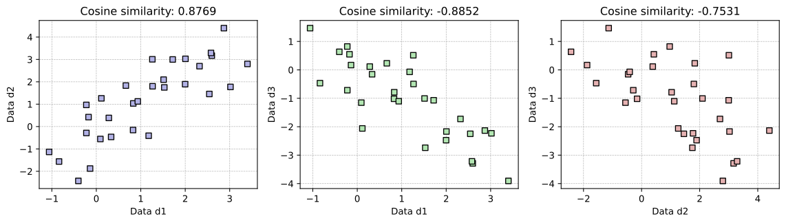
Key Take-home Points
- Geometric Interpretation: Cosine similarity measures the angle between two vectors, ranging from -1 (opposite) to 1 (identical).
- Magnitude Invariant: Unlike Euclidean distance, cosine similarity is not affected by the magnitude (length) of the vectors, only their direction.
- Pearson Connection: When vectors are mean-centered, their cosine similarity equals their Pearson correlation coefficient.
- Framework Support: Both Sklearn and PyTorch provide optimized functions for computing similarity, which is a core operation in modern NLP.