Adapted from A deep understanding of AI language model mechanisms — https://udemy.com/course/dullms_x
1. Setup and Environment
We'll start by importing our standard visualization tools and configuring the plotting backend for high-quality SVG outputs.
import numpy as np
import matplotlib.pyplot as plt
from matplotlib.gridspec import GridSpec

import matplotlib_inline.backend_inline
matplotlib_inline.backend_inline.set_matplotlib_formats('svg')
2. Loading GPT-2
In this lesson, we use the GPT-2 model and tokenizer to explore how subword tokens relate to each other in the embedding space.
from transformers import GPT2Model,GPT2Tokenizer

# pretrained GPT-2 model and tokenizer
gpt2 = GPT2Model.from_pretrained('gpt2')
tokenizer = GPT2Tokenizer.from_pretrained('gpt2')/Users/drippy/.pyenv/versions/3.12.6/lib/python3.12/site-packages/tqdm/auto.py:21: TqdmWarning: IProgress not found. Please update jupyter and ipywidgets. See https://ipywidgets.readthedocs.io/en/stable/user_install.html
from .autonotebook import tqdm as notebook_tqdmMatrix Extraction
We extract the Word Token Embeddings (WTE) matrix to analyze the learned 768-dimensional vectors for all 50,257 tokens.
# get the Word Token Embeddings matrix
embeddings = gpt2.wte.weight.detach().numpy()
3. Subword Tokenization Analysis
GPT-2 uses BPE tokenization, which often breaks common words into multiple sub-tokens. Let's see how words like "banana" and "cosmic" are decomposed.
# words of interest
word1 = 'banana'
word2 = 'apple'
word3 = 'cosmic'

# decomposition
for w in [word1,word2,word3]:
  t = tokenizer.encode(w)
print(f'"{w}" comprises {len(t)} tokens:\n {[tokenizer.decode(i) for i in t]}\n')"banana" comprises 2 tokens:
['ban', 'ana']
"apple" comprises 1 tokens:
['apple']3 more lines
"cosmic" comprises 2 tokens:
   ['cos', 'mic']
Visualizing Subword Embeddings
By plotting the vectors of sub-tokens like "ban" and "ana," we can see if parts of the same word share similar semantic "fingerprints."
# setup the figure subplot geometry
fig = plt.figure(figsize=(10,7))
gs = GridSpec(2,2)
ax0 = fig.add_subplot(gs[0,:])
ax1 = fig.add_subplot(gs[1,0])
ax2 = fig.add_subplot(gs[1,1])


# plot the embeddings by dimension
colors = 'krb'
linestyles = ['-','--','-.',':']
for idx,word in enumerate([word1,word2,word3]):
  wordidx = tokenizer.encode(word)
  for j in range(len(wordidx)):
    ax0.plot(embeddings[wordidx[j],:],linestyle=linestyles[j],color=colors[idx],label=tokenizer.decode(wordidx[j]))

ax0.set(xlabel='Dimension',title='Embeddings',xlim=[-1,embeddings.shape[1]+1])
ax0.legend()


# cosine similarity between 'ban' and 'ana'
v1 = embeddings[tokenizer.encode('ban')]
v2 = embeddings[tokenizer.encode('ana')]
cossim = np.sum(v1*v2)/(np.linalg.norm(v1)*np.linalg.norm(v2))

# plot the embeddings by each other
ax1.plot(v1,v2,'ko',markerfacecolor=[.7,.7,.7,.6])
ax1.set(xlim=[-.8,.8],ylim=[-.8,.8],xlabel='"ban" embedding',ylabel='"ana" embedding',
        title=f'Cosine similarity = {cossim:.3f}')


# plot the "cos" for two endings
for s in ['mic','ine']:

  # cosine similarity
  v1 = embeddings[tokenizer.encode('cos')].squeeze()
  v2 = embeddings[tokenizer.encode(s)].squeeze()
  cossim = np.sum(v1*v2) / (np.linalg.norm(v1)*np.linalg.norm(v2))

  # plot
  ax2.plot(v1,v2,marker=f'${s[0]}$',linestyle='none',alpha=.6,label=f'cos-{s} ($s_c$  = {cossim:.3f})')

ax2.legend(fontsize=10)
ax2.set(xlim=[-.8,.8],ylim=[-.8,.8],xlabel='"cos" embedding',ylabel='"mic" or "ine" embedding')


# final touches
plt.tight_layout()
plt.show()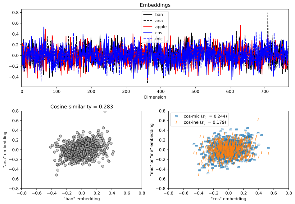
4. Finding Semantic Neighbors
We can find the most similar tokens to a seed word (like "Mike") by calculating the cosine similarity between its vector and every other vector in the model.
# get seed index and embedding vector
seed = tokenizer.encode('Mike')
seedvect = embeddings[seed].squeeze()
seedvectNorm = np.linalg.norm(seedvect)

# calculate cosine similarity to all other tokens in a for-loop
cossims = np.zeros(embeddings.shape[0])
for idx,v in enumerate(embeddings):
  cossims[idx] = np.sum(seedvect*v) / (seedvectNorm*np.linalg.norm(v))


# and visualize
plt.figure(figsize=(10,4))
plt.plot(cossims,'k.',alpha=.6,markerfacecolor='w')
plt.gca().set(xlim=[-5,len(cossims)+5],xlabel='Token index',ylabel='Cosine similarity',
              title='Cosine similarity to "Mike"')


# top 20 largest cosine-similarities
top20 = np.argsort(cossims)[-20:]
for i in top20:
  plt.plot(i,cossims[i],'ms',markersize=4,alpha=.6)

plt.show()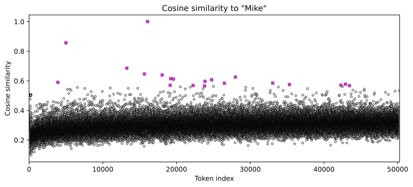
Identifying Similar Tokens
Let's print the top 20 most similar tokens. Notice how the model groups different names and variations of the same name together.
# tokens closest to "Mike"
for n in top20[::-1]:
print(f'"{tokenizer.decode(n)}" with cosine similarity {cossims[n]:.3f}')"Mike" with cosine similarity 1.000
" Mike" with cosine similarity 0.857
"Michael" with cosine similarity 0.685
"Chris" with cosine similarity 0.647
"Jim" with cosine similarity 0.64015 more lines
"Dave" with cosine similarity 0.626
"Steve" with cosine similarity 0.615
"Joe" with cosine similarity 0.612
"Brian" with cosine similarity 0.607
"Kevin" with cosine similarity 0.597
" Michael" with cosine similarity 0.590
"Rick" with cosine similarity 0.585
"Jason" with cosine similarity 0.584
"Larry" with cosine similarity 0.578
"Andy" with cosine similarity 0.575
"Doug" with cosine similarity 0.570
"Jeff" with cosine similarity 0.570
"Richard" with cosine similarity 0.569
"Jerry" with cosine similarity 0.568
"Josh" with cosine similarity 0.566
5. Vectorized Similarity Calculation
For-loops are slow in Python. We can use linear algebra (matrix-vector multiplication) to calculate all cosine similarities simultaneously for a massive speedup.
# normalize entire embedding matrix (in a new variable!)
Enorm = embeddings / np.linalg.norm(embeddings,axis=1,keepdims=True)

# cosine similarity matrices
cossims2 = Enorm[seed] @ Enorm.Tprint(f'Size of for-loop version: {cossims.shape}')
print(f'Size of vectorized version: {cossims2.shape}')
# remove singleton dimension
cossims2 = np.squeeze(cossims2)
# inspect again
print('\n** After squeezing:')
print(f'Size of for-loop version: {cossims.shape}')
print(f'Size of vectorized version: {cossims2.shape}')Size of for-loop version: (50257,)
Size of vectorized version: (1, 50257)
** After squeezing:
Size of for-loop version: (50257,)1 more line
Size of vectorized version: (50257,)Verifying Results
Finally, we'll plot the results from both the for-loop and the vectorized versions to ensure they are identical and highly correlated.
plt.figure(figsize=(10,4))
plt.plot(range(0,len(cossims),100),cossims[::100],'o',label='for-loop')
plt.plot(range(0,len(cossims),100),cossims2[::100],'+',label='vectorized')

plt.legend()
plt.gca().set(xlabel='Token idx (plotting every 100)',ylabel='Cossine similarity',title=f'Correlation = {np.corrcoef(cossims,cossims2)[0,1]:.3f}')
plt.show()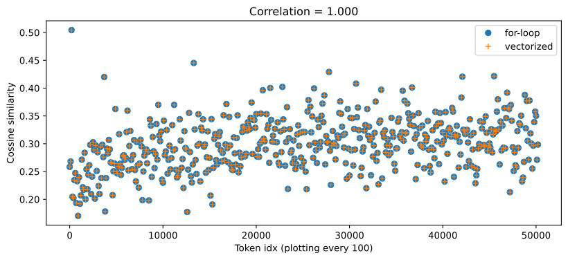
Key Take-home Points
- Subword Relations: Tokens that form the same word (e.g., "ban" and "ana") often have distinct but related embedding vectors.
- Semantic Clusters: GPT-2's embedding space naturally clusters similar concepts like names (Mike, Michael, Chris) without explicit supervision.
- Linear Algebra Speed: Vectorizing similarity calculations using matrix multiplication is significantly faster than using Python for-loops.
- Normalization: Proper normalization (scaling vectors to unit length) is crucial when calculating cosine similarity via dot products.