Adapted from A deep understanding of AI language model mechanisms — https://udemy.com/course/dullms_x
1. Setup and Libraries
We'll begin by importing our text processing and deep learning libraries. We'll also use torchinfo to visualize our model's architecture and parameters.
# typical libraries...
import numpy as np
import matplotlib.pyplot as plt
import matplotlib as mpl

# for importing and working with texts
import requests
import re
import string

# pytorch stuff
from torch.utils.data import Dataset, DataLoader
import torch
import torch.nn as nn
import torch.nn.functional as F

!pip install torchinfo # not installed by default in colab
from torchinfo import summary

import matplotlib_inline.backend_inline
matplotlib_inline.backend_inline.set_matplotlib_formats('svg')Requirement already satisfied: torchinfo in /Users/drippy/.pyenv/versions/3.12.6/lib/python3.12/site-packages (1.8.0)
[notice] A new release of pip is available: 25.1.1 -> 26.1.1
[notice] To update, run: pip install --upgrade pipCode below is for video "Create a data loader to train a model"
2. Text Preprocessing
We'll download a classic text (H.G. Wells' The Time Machine) and clean it by removing special characters, numbers, and converting everything to lowercase.
# get raw text from internet (The Time Machine... yeah I use it a lot :P  )
text = requests.get('https://www.gutenberg.org/files/35/35-0.txt').text
# character strings to replace with space
strings2replace = [ '\r\n\r\nâ\x80\x9c','â\x80\x9c','â\x80\x9d','\r\n','â\x80\x94','â\x80\x99','â\x80\x98','_', ]

# use regular expression (re) to replace those strings with space
for str2match in strings2replace:
  text = re.compile(r'%s'%str2match).sub(' ',text)

# remove non-ASCII characters and numbers, and make lower-case
text = re.sub(r'[^\x00-\x7F]+', ' ', text)
text = re.sub(r'\d+','',text).lower()

# split into words with >1 letter
words = re.split(fr'[{string.punctuation}\s]+',text)
words = [item.strip() for item in words if item.strip()]
words = [item for item in words if len(item)>1]
3. Creating the Vocabulary
After cleaning, we create a mapping between words and unique integer IDs. We then generate overlapping sequences to serve as our input and target data.
# create the vocabulary (lexicon)
vocab  = sorted(set(words))
nWords = len(words)
nVocab = len(vocab)

# encoder/decoder look-up-tables (as python dictionaries)
word2idx = {w:i for i,w in enumerate(vocab)}
idx2word = {i:w for i,w in enumerate(vocab)}

# show a few keys in the dictionary
print(f'The book contains {nWords:,} words, {nVocab:,} of which are unique and comprise the vocab.')
print(f'\n\nFirst 10 vocab words:\n',list(word2idx.keys())[:10])<>:12: SyntaxWarning: invalid escape sequence '\d'
<>:15: SyntaxWarning: invalid escape sequence '\s'
<>:12: SyntaxWarning: invalid escape sequence '\d'
<>:15: SyntaxWarning: invalid escape sequence '\s'
/var/folders/41/x856_7w17ss36djfjfjccwcr0000gn/T/ipykernel_94798/2659864497.py:12: SyntaxWarning: invalid escape sequence '\d'3 more lines
  text = re.sub('\d+','',text).lower()
/var/folders/41/x856_7w17ss36djfjfjccwcr0000gn/T/ipykernel_94798/2659864497.py:15: SyntaxWarning: invalid escape sequence '\s'
words = re.split(f'[{string.punctuation}\s]+',text)The book contains 30,698 words, 4,589 of which are unique and comprise the vocab.
First 10 vocab words:
['abandon', 'abandoned', 'able', 'abnormally', 'abominable', 'abominations', 'about', 'above', 'abruptly', 'absence']# parameters for dataset
context_length = 8 # context length
stride = 2 # skipping
# initialize
inputs = []
targets = []
# overlapping sequences of context_length
for i in range(0,nWords-context_length,stride):
# get a few words
in_seq = words[i : i+context_length ]
targ_seq = words[i+1: i+context_length+1]
# append to the lists
inputs.append([word2idx[w] for w in in_seq])
targets.append([word2idx[w] for w in targ_seq])
print(inputs[123])
print(targets[123])[1342, 4304, 4119, 342, 4296, 3388, 1474, 131]
[4304, 4119, 342, 4296, 3388, 1474, 131, 209]# a closer look:
print('Inputs: ',inputs[4])
print('Targets:',targets[4])
print('')
print('Inputs :',inputs[5])
print('Targets:',targets[5])
# this is what we need, although we need it in torch Dataset/DataLoader formatInputs: [2416, 131, 2172, 506, 4451, 783, 2167, 2005]
Targets: [131, 2172, 506, 4451, 783, 2167, 2005, 4042]
Inputs : [2172, 506, 4451, 783, 2167, 2005, 4042, 2416]
Targets: [506, 4451, 783, 2167, 2005, 4042, 2416, 2006]# we need each list to be a tensor
torch.tensor(inputs[4])tensor([2416, 131, 2172, 506, 4451, 783, 2167, 2005])4. Dataset and Dataloader
We'll encapsulate our data logic into a custom PyTorch Dataset class and use a DataLoader to handle batching and shuffling during training.
# create a class for a dataset
class WordDataset(Dataset):
  def __init__(self, text, word2idx, context_length=8, stride=4):

    # initialize
    self.inputs  = []
    self.targets = []
    self.word2idx = word2idx  # stored locally in the object

    # overlapping sequences of context_length
    for i in range(0,len(text)-context_length,stride):

      # get a few words
      in_seq   = text[i : i+context_length]
      targ_seq = text[i+1 : i+context_length+1]

      # append to the lists
      self.inputs.append(torch.tensor([word2idx[w] for w in in_seq]))
      self.targets.append(torch.tensor([word2idx[w] for w in targ_seq]))

  def __len__(self):
    return len(self.inputs)

  def __getitem__(self, idx):
    return self.inputs[idx], self.targets[idx]


# create an instance!
context_length = 6 # context length
stride = 3 # skipping over tokens
text_dataset = WordDataset(words,word2idx,context_length,stride)

text_dataset[4](tensor([4451, 783, 2167, 2005, 4042, 2416]),
tensor([ 783, 2167, 2005, 4042, 2416, 2006]))And a dataloader for training
# also need a dataloader
dataloader = DataLoader(
                text_dataset,
                batch_size = 32, # 2 for looking; 32 for training
                shuffle    = True,
                drop_last  = True
            )

# let's have a look at the indices
X,y = next(iter(dataloader))
print('Inputs:')
print(X), print('')

print('Targets:')
print(y), print('\n\n\n')

# and the words
print('Inputs in words (first batch):')
print([idx2word[item.item()] for item in X[0]])
print('')

print('Targets in words (first batch):')
print([idx2word[item.item()] for item in y[0]])Inputs:
tensor([[1466, 151, 255, 3502, 151, 255],
[4051, 2468, 2741, 1861, 339, 1815],
[1868, 1815, 3468, 255, 495, 501],
[3116, 2186, 1122, 137, 4047, 2186],71 more lines
        [3229, 2186,  230, 3332, 3102, 2731],
        [3176, 1338, 1474,  332, 2886,  664],
        [1298, 4041, 3554, 2210,  255, 4042],
        [4073,  255,   96,   91, 2069, 4051],
        [3613, 2007, 2364, 4042, 1533, 2731],
        [3275, 3865, 2731,  774, 2669, 2638],
        [2764, 4042, 2861, 1111, 1572,  580],
        [1929, 1869, 1868, 3771, 2347, 2742],
        [3915, 3546, 4363, 1353, 2191, 4042],
        [4009,  137,   74, 1752, 1465, 4556],
        [ 289, 4296, 4042, 1018,  255, 2275],
        [4119, 2609,  137, 2608,  877, 4408],
        [3843, 1317, 2470,  137, 4395,  280],
        [2741, 2569, 1572, 4042,  839, 2595],
        [4041,  519,  151, 4077, 2387,  255],
        [2347, 1977, 3759, 2186, 4408,  651],
        [1495,  255, 4042,  472, 2832, 4077],
        [3321, 1769, 4041, 2742, 3469, 2740],
        [1019,  230, 4042, 2563,  850, 4295],
        [2583, 1645, 2673, 1929, 1869, 1708],
        [ 443, 4352, 3720, 1815,  629, 3684],
        [2041, 2946, 4510, 2230, 2731, 2933],
        [2477, 1815, 3468, 2041, 4042, 4254],
        [ 576, 2731, 4042, 1826, 4458, 4408],
        [ 125, 4042, 1790, 3401, 4042, 1973],
        [4252, 4041, 4428, 4454, 3463, 3225],
        [4581, 3183, 1696, 4045, 3388, 4042],
        [4478,  137, 1815, 3854, 2270, 1775]])

Targets:
tensor([[ 151,  255, 3502,  151,  255, 4222],
        [2468, 2741, 1861,  339, 1815, 3359],
        [1815, 3468,  255,  495,  501,  340],
        [2186, 1122,  137, 4047, 2186,  519],
        [2186,  230, 3332, 3102, 2731, 1977],
        [1338, 1474,  332, 2886,  664, 4042],
        [4041, 3554, 2210,  255, 4042, 1998],
        [ 255,   96,   91, 2069, 4051, 4408],
        [2007, 2364, 4042, 1533, 2731, 2186],
        [3865, 2731,  774, 2669, 2638, 2731],
        [4042, 2861, 1111, 1572,  580, 2243],
        [1869, 1868, 3771, 2347, 2742, 4481],
        [3546, 4363, 1353, 2191, 4042, 2572],
        [ 137,   74, 1752, 1465, 4556,  137],
        [4296, 4042, 1018,  255, 2275, 3406],
        [2609,  137, 2608,  877, 4408,  255],
        [1317, 2470,  137, 4395,  280,   71],
        [2569, 1572, 4042,  839, 2595, 2731],
        [ 519,  151, 4077, 2387,  255, 4042],
        [1977, 3759, 2186, 4408,  651, 1122],
        [ 255, 4042,  472, 2832, 4077, 1880],
        [1769, 4041, 2742, 3469, 2740, 1581],
        [ 230, 4042, 2563,  850, 4295, 4042],
        [1645, 2673, 1929, 1869, 1708, 3538],
        [4352, 3720, 1815,  629, 3684, 1487],
        [2946, 4510, 2230, 2731, 2933, 3379],
        [1815, 3468, 2041, 4042, 4254, 2186],
        [2731, 4042, 1826, 4458, 4408,  664],
        [4042, 1790, 3401, 4042, 1973, 3272],
        [4041, 4428, 4454, 3463, 3225, 4051],
        [3183, 1696, 4045, 3388, 4042, 2481],
        [ 137, 1815, 3854, 2270, 1775, 3209]])


Inputs in words (first batch):
['fifteen', 'another', 'at', 'seventeen', 'another', 'at']

Targets in words (first batch):
['another', 'at', 'seventeen', 'another', 'at', 'twenty']
Code below is for video "Build a model to learn the embeddings"
5. Embedding Dimensionality Heuristics
How many dimensions should an embedding space have? We'll explore common heuristics used for mapping vocabulary size to optimal vector dimensions.
# exploring dimensionality based on vocab sizes

# vocab sizes
N = np.logspace(np.log10(1000),np.log10(100000),23)

# heuristic for non-LLM models like word2vec or glove:
embdim = np.sqrt(N)

# parameters for GPT2
gpt2dims = [ 50257,768 ]

plt.figure(figsize=(8,4))

# heuristic line
plt.plot(N,embdim,'ks-',markersize=8,markerfacecolor=[.9,.7,.7],label=r'$s = \sqrt{N}$')

# expected embedding dim for GPT2
plt.plot([gpt2dims[0],gpt2dims[0]],[0,np.sqrt(gpt2dims[0])],'k--',linewidth=1,label='Expected GPT2')
plt.plot([0,gpt2dims[0]],[np.sqrt(gpt2dims[0]),np.sqrt(gpt2dims[0])],'k--',linewidth=1)

# actual GPT2 embedding
plt.plot([gpt2dims[0],gpt2dims[0]],[0,gpt2dims[1]],'b:',linewidth=1,label='Actual GPT2')
plt.plot([0,gpt2dims[0]],[gpt2dims[1],gpt2dims[1]],'b:',linewidth=1)

plt.gca().set(xlabel='Vocab size',ylabel='Embeddings dimensions',
              xlim=[-100,N[-1]+2000],ylim=[0,None])
plt.legend()
plt.show()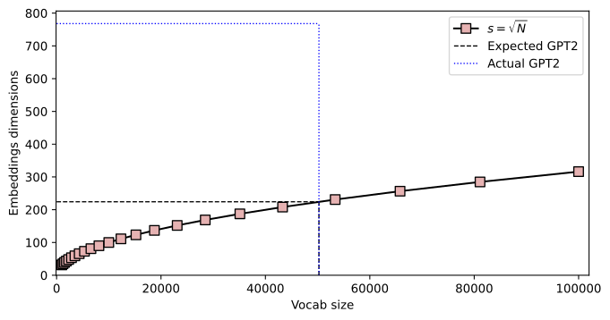
6. Creating an Embedding Layer
We'll initialize a random embedding layer using nn.Embedding and visualize its structure. At this stage, the weights are purely random and have no semantic meaning.
# dimensionality of embedding space (arbitrarily set to 100)
embeddingDimension = 100

# create a random embedding
embedding_layer = nn.Embedding(nVocab,embeddingDimension)

# let's see its size
embedding_layer.weight.shapetorch.Size([4589, 100])# what does it look like?
_,axs = plt.subplots(1,2,figsize=(12,4))
axs[0].imshow(embedding_layer.weight.detach().T,aspect='auto',vmin=-1,vmax=1)
axs[0].set(ylabel='Embedding dimension',xlabel='Token index',title='Entire embedding matrix')
# pick a word at random
aRandomWord = np.random.choice(vocab)
# plot its embedding
axs[1].plot(embedding_layer.weight.detach()[word2idx[aRandomWord],:],'ks',markerfacecolor=[.7,.9,.7])
axs[0].axvline(word2idx[aRandomWord],color='w',linestyle='--')
axs[1].set(xlabel='Embedding dimension',ylabel='Weight value',title=f'Embedding for "{aRandomWord}" (idx = {word2idx[aRandomWord]})')
plt.tight_layout()
plt.show()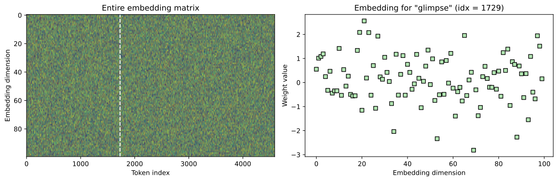
# embeddings for closely related words
word1 = 'time'
word2 = 'machine'

# their embeddings
embed1 = embedding_layer.weight.detach()[word2idx[word1],:]
embed2 = embedding_layer.weight.detach()[word2idx[word2],:]

# cosine similiarity between them
cosSim = torch.dot(embed1,embed2)/(torch.norm(embed1)*torch.norm(embed2))

# vizualize
plt.plot(embed1,embed2,'ks',markerfacecolor=[.7,.9,.7],alpha=.6)
plt.gca().set(xlabel=f'Embedding for "{word1}"',ylabel=f'Embedding for "{word2}"',
              title=f'Cosine similarity: {cosSim:.3f}')
plt.show()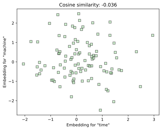
7. Embedding Model Architecture
Our training model consists of an embedding layer followed by two linear layers and a log-softmax output for token classification.
class EmbeddingModel(nn.Module):
  def __init__(self, vocab_size, embedding_dim, context_size):
    super(EmbeddingModel, self).__init__()

    # embedding layer
    self.embeddings = nn.Embedding(vocab_size, embedding_dim)

    # linear layers
    self.linear1 = nn.Linear(context_size * embedding_dim, 128)
    self.linear2 = nn.Linear(128, vocab_size)

  def forward(self, inputs):

    # extract and flatten embeddings [batch_size, context_size * embedding_dim]
    embeds = self.embeddings(inputs).view(inputs.shape[0],-1)

    # fully connected layers
    out = F.relu(self.linear1(embeds))
    out = self.linear2(out)

    # log softmax for classification (note: NLLLoss expects logprobs as inputs)
    log_probs = F.log_softmax(out, dim=1)
    return log_probs


# create a model instance!
model = EmbeddingModel(vocab_size=nVocab, embedding_dim=embeddingDimension, context_size=context_length)
print(model)

# apply Xavier weight distribution
for param in model.parameters():
  if param.dim()>1: # also excludes biases
nn.init.xavier_normal_(param)EmbeddingModel(
(embeddings): Embedding(4589, 100)
(linear1): Linear(in_features=600, out_features=128, bias=True)
(linear2): Linear(in_features=128, out_features=4589, bias=True)
)# let's test the model
X,y = next(iter(dataloader))
modelOut = model(X)
print('Input to model:')
print(X), print('')
print(f'Output from model (size: {list(modelOut.detach().shape)}):')
print(modelOut)Input to model:
tensor([[3195, 2368, 1640, 2608, 2518, 4119],
[ 425, 2731, 2780, 4544, 4408, 1742],
[4171, 1857, 4119, 1861, 3494, 4388],
[4042, 2190, 308, 2183, 832, 137],38 more lines
        [ 501, 3712, 3831, 1408,  729, 4581],
        [2988, 4461, 4428,  196, 2186,    6],
        [1354, 1572, 4073, 4041, 1556, 4275],
        [4119, 4042, 4340, 4146, 4119, 4042],
        [4510,  410, 4581, 4481, 1861, 2651],
        [3086,  506, 2368,  874, 1640, 4042],
        [ 339, 3888,  148,  987, 2597, 2041],
        [1230, 1981,  137, 4230, 4079, 3501],
        [4495, 2585, 1424,  137, 1424, 4144],
        [ 497,   48,  137,  886, 2358, 2731],
        [2186, 4408, 2685, 2698, 3913, 4352],
        [2163, 2608, 1385, 4042,    9, 1640],
        [4529, 4454,  131,  110, 2653,  137],
        [4066, 2731,   96, 4041,  350, 2041],
        [1594, 3693, 3975, 2740, 2608, 3330],
        [4109, 4171, 3116, 1929, 1832, 4119],
        [4057, 4042, 2569, 3693,  230, 1572],
        [2685,  131, 1196, 1258, 4538, 2369],
        [4408, 3652, 2347, 4327, 4092, 4042],
        [4119, 3192, 4042, 1586, 2731, 2186],
        [2470, 3819,  230, 2186, 3304, 2186],
        [ 921,  817, 2685, 1297, 3400, 2609],
        [ 896, 2731, 4042, 3507, 1971, 4428],
        [4039, 4042, 4297,  137, 4461, 2778],
        [1125, 4454, 2008,  255, 1492, 4428],
        [2569, 1096, 2186, 4408, 4352, 2270],
        [2155, 2183, 2186,   84,   84, 3388],
        [4466, 2183, 1166, 4119, 4042, 2315]])

Output from model (size: [32, 4589]):
tensor([[-8.4354, -8.4701, -8.3825,  ..., -8.4494, -8.4092, -8.5281],
        [-8.4361, -8.4760, -8.3863,  ..., -8.4454, -8.4117, -8.5215],
        [-8.4348, -8.4726, -8.3785,  ..., -8.4426, -8.4032, -8.5260],
        ...,
        [-8.4366, -8.4713, -8.3677,  ..., -8.4487, -8.4084, -8.5308],
        [-8.4286, -8.4730, -8.3732,  ..., -8.4468, -8.4078, -8.5306],
        [-8.4378, -8.4740, -8.3749,  ..., -8.4521, -8.4016, -8.5309]],
grad_fn=<LogSoftmaxBackward0>)# log soft-max output:
print(modelOut.detach()[0])
print('')
# shouldn't the sum be 1?
print(f'Log softmax sum = {modelOut.detach()[0].sum():.3f}')
# ah, it's *log* softmax :D
print(f'exp(log(softmax)) sum = {torch.exp(modelOut.detach()[0]).sum():.3f}')tensor([-8.4354, -8.4701, -8.3825, ..., -8.4494, -8.4092, -8.5281])
Log softmax sum = -38697.754
exp(log(softmax)) sum = 1.000# find the word with the highest probability
print('Model input:')
print([idx2word[w.item()] for w in X[0]])
print('')
print('Model output:')
print(idx2word[modelOut[0].argmax().item()])Model input:
['receded', 'little', 'from', 'my', 'mind', 'to']
Model output:
deadlyplt.plot(modelOut[0].detach(),'o');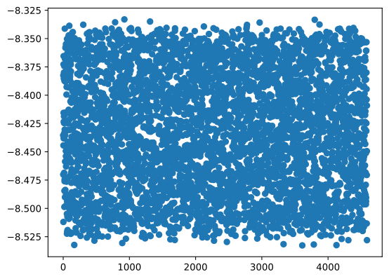
8. Initial Text Generation (Untrained)
Before training, we'll ask the model to generate a sequence. Since the weights are random, the output will be semantically meaningless "word salad."
# grab some data from the loader
X,y = next(iter(dataloader))

print('First input:')
print(' '.join([idx2word[w.item()] for w in X[0]]))
print('\nSubsequent inputs:')

# text generation
for _ in range(context_length):

  # get output for this input
  Y = model(X)

  # pick the most likely next word
  nextWord = Y[0].argmax().item()

  # create new input for the next iteration (word)
  X[0] = torch.concatenate((X[0][1:],torch.tensor([nextWord])))

  # print out the generated text so far
print(' '.join([idx2word[w.item()] for w in X[0]]))First input:
shape of rare fossils broken to
Subsequent inputs:
of rare fossils broken to deadly5 more lines
rare fossils broken to deadly shower
fossils broken to deadly shower bar
broken to deadly shower bar ancestors
to deadly shower bar ancestors geometrical
deadly shower bar ancestors geometrical diet
How big is our model?
# summary of model and parameters
summary(model, input_data=X, col_names=['input_size','output_size','num_params'])===================================================================================================================
Layer (type:depth-idx) Input Shape Output Shape Param #
===================================================================================================================
EmbeddingModel [32, 6] [32, 4589] --
├─Embedding: 1-1 [32, 6] [32, 6, 100] 458,90013 more lines
├─Linear: 1-2                            [32, 600]                 [32, 128]                 76,928
├─Linear: 1-3                            [32, 128]                 [32, 4589]                591,981
===================================================================================================================
Total params: 1,127,809
Trainable params: 1,127,809
Non-trainable params: 0
Total mult-adds (Units.MEGABYTES): 36.09
===================================================================================================================
Input size (MB): 0.00
Forward/backward pass size (MB): 1.36
Params size (MB): 4.51
Estimated Total Size (MB): 5.87
===================================================================================================================
Code below is for video "Train and evaluate the model"
# we'll use the GPU for speed
device = torch.device('cuda' if torch.cuda.is_available() else 'cpu')
print(f'Using device: {device}')Using device: cpu# create a fresh model instance
model = EmbeddingModel(vocab_size=nVocab, embedding_dim=embeddingDimension, context_size=context_length)
# with Xavier weight distribution
for param in model.parameters():
if param.dim()>1: nn.init.xavier_normal_(param)
# and move it to the GPU
model = model.to(device)# create the loss and optimizer functions
loss_function = nn.NLLLoss().to(device)
optimizer = torch.optim.AdamW(model.parameters(), lr=.001, weight_decay=.01)# quick test for errors and sanity-check the output matrix sizes
X,y = next(iter(dataloader))
X,y = X.to(device), y.to(device)
# forward pass
modelOutput = model(X)
# check the sizes
print(f'Model input is of size: {X.shape}')
print(f'Target output is of size: {y.shape}')
print(f'Model output is of size: {modelOutput.shape}')
# loss function
loss = loss_function(modelOutput,y[:,-1])
print(f'\nLoss:')
lossModel input is of size: torch.Size([32, 6])
Target output is of size: torch.Size([32, 6])
Model output is of size: torch.Size([32, 4589])
Loss:tensor(8.4298, grad_fn=<NllLossBackward0>)# extract a copy of the pretrained embedding weights for comparison later
pretrained_embeddings = model.embeddings.weight.detach().cpu().clone()# reminder: use batchsize=32 in data loader ;)9. Training the Model
We define our training loop, move the model to the GPU (if available), and use the AdamW optimizer to minimize the negative log-likelihood loss.
def trainTheModel(model,num_epochs=25):

  # initialize losses
  total_loss = np.zeros(num_epochs)

  for epoch in range(num_epochs):

    # initialize
    epoch_loss = 0

    # loop over batches in the data loader
    for X,y in dataloader:

      # move data to GPU
      X,y = X.to(device), y.to(device)

      # clear previous gradients
      model.zero_grad()

      # forward pass
      log_probs = model(X)

      # calculate the losses from the final target word
      loss = loss_function(log_probs,y[:,-1])

      # backprop
      loss.backward()
      optimizer.step()

      # sum the per-epoch losses
      epoch_loss += loss.item()

    # scale by the number of tokens in this dataloader
    total_loss[epoch] = epoch_loss / len(dataloader.dataset)

    # update our progress :)
    print(f'  Finished epoch {epoch+1} with loss {epoch_loss / len(dataloader.dataset):.4f}')

  # output the model and the losses
return model,total_loss# train the model!
model,total_loss = trainTheModel(model) # using default 25 epochs
# plot the losses
plt.figure(figsize=(10,3))
plt.plot(total_loss,'ks-',markerfacecolor='w',markersize=8)
plt.gca().set(xlabel='Epoch',ylabel='Loss')
plt.show() Finished epoch 1 with loss 0.2170
Finished epoch 2 with loss 0.1879
Finished epoch 3 with loss 0.1749
Finished epoch 4 with loss 0.1635
Finished epoch 5 with loss 0.152820 more lines
  Finished epoch 6 with loss 0.1414
  Finished epoch 7 with loss 0.1287
  Finished epoch 8 with loss 0.1142
  Finished epoch 9 with loss 0.0981
  Finished epoch 10 with loss 0.0803
  Finished epoch 11 with loss 0.0612
  Finished epoch 12 with loss 0.0421
  Finished epoch 13 with loss 0.0254
  Finished epoch 14 with loss 0.0138
  Finished epoch 15 with loss 0.0071
  Finished epoch 16 with loss 0.0037
  Finished epoch 17 with loss 0.0021
  Finished epoch 18 with loss 0.0012
  Finished epoch 19 with loss 0.0009
  Finished epoch 20 with loss 0.0006
  Finished epoch 21 with loss 0.0005
  Finished epoch 22 with loss 0.0004
  Finished epoch 23 with loss 0.0003
  Finished epoch 24 with loss 0.0003
  Finished epoch 25 with loss 0.0003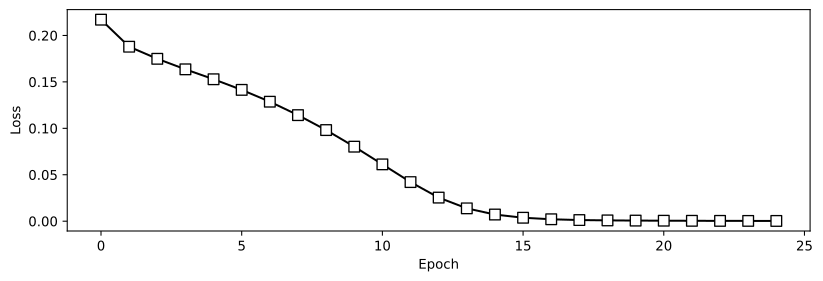
# get a copy of the trained weights
postrained_embeddings = model.embeddings.weight.detach().cpu().clone()# Plenty of empty space so you won't look by accident :PCode below is for video "CodeChallenge: How the embeddings change"
Exercise 1: distributions of embeddings
10. Analyzing Weight Changes
How much did the embeddings actually change during training? We'll compare the weight distributions before and after the 25 epochs of optimization.
# histograms via numpy
yPre,xPre = np.histogram(pretrained_embeddings.flatten(),bins=50)
yPst,xPst = np.histogram(postrained_embeddings.flatten(),bins=50)

# recalculate x values as bin centers
xPre = (xPre[1:]+xPre[:-1]) / 2
xPst = (xPst[1:]+xPst[:-1]) / 2

# and plot
plt.figure(figsize=(12,5))
plt.bar(xPst,yPst,width=xPst[1]-xPst[0],color=[.7,.9,.7,.7],edgecolor=[.3,.6,0,.4],label='POSTtrain')
plt.bar(xPre,yPre,width=xPre[1]-xPre[0],color=[.9,.7,.7,.3],edgecolor=[.6,0,.3,.4],label='PREtrain')

plt.gca().set(xlabel='Weight value',ylabel='Count',title='Distributions of embedding weights')
plt.legend()
plt.show()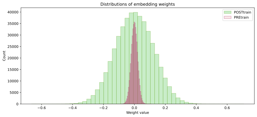
Exercise 2: Embeddings vectors for a random word
# pick a word at random
aRandomWord = np.random.choice(vocab)
randWord_idx = word2idx[aRandomWord]

# extract its embeddings vectors
pre_ev = pretrained_embeddings[randWord_idx,:]
pst_ev = postrained_embeddings[randWord_idx,:]


_,axs = plt.subplots(2,2,figsize=(10,7))

# the pretrainined embeddings
axs[0,0].imshow(pretrained_embeddings.T,aspect='auto',vmin=-.2,vmax=.2)
axs[0,0].set(ylabel='Embedding dimension',xlabel='Token index',title='PREtrain embedding matrix')

# the post-trainined embeddings
axs[0,1].imshow(postrained_embeddings.T,aspect='auto',vmin=-.2,vmax=.2)
axs[0,1].set(ylabel='Embedding dimension',xlabel='Token index',title='POSTtrain embedding matrix')


axs[0,0].axvline(randWord_idx,linestyle='--',color=[.8,.8,.8])
axs[0,1].axvline(randWord_idx,linestyle='--',color=[.8,.8,.8])

# plot its embedding
axs[1,0].plot(pre_ev,'ks-',markerfacecolor=[.7,.9,.7],label='PREtrain')
axs[1,0].plot(pst_ev,'ko-',markerfacecolor=[.9,.7,.7],label='POSTtrain')
axs[1,0].set(xlabel='Embedding dimension',ylabel='Weight value',title=f'"{aRandomWord}" embedding (idx={randWord_idx})')
axs[1,0].legend(fontsize=8)

# how it changed
axlim = max(abs(pre_ev).max(),abs(pst_ev).max()) * 1.1 # equal axis limits
axs[1,1].plot(pre_ev,pst_ev,'ks',markerfacecolor=[.9,.7,.9])
axs[1,1].set(xlim=[-axlim,axlim],ylim=[-axlim,axlim],xlabel='PREtrain embedding',
             ylabel='POSTtrain embedding',title='Change in embedding')

plt.tight_layout()
plt.show()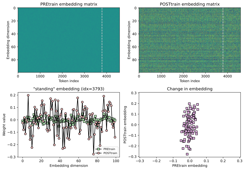
Exercise 3: Time Machine embeddings
# embeddings for closely related words
word1 = 'time'
word2 = 'machine'

# their embeddings
embed1pre = pretrained_embeddings[word2idx[word1],:]
embed2pre = pretrained_embeddings[word2idx[word2],:]
embed1pst = postrained_embeddings[word2idx[word1],:]
embed2pst = postrained_embeddings[word2idx[word2],:]

# cosine similarity between them
cosSim_pre = F.cosine_similarity(embed1pre.unsqueeze(dim=0),embed2pre.view(1,-1))
cosSim_pst = nn.functional.cosine_similarity(embed1pst.unsqueeze(dim=0),embed2pst.view(1,-1))


# vizualize
_,axs = plt.subplots(1,2,figsize=(10,4))

axlim = torch.cat((abs(embed1pre),abs(embed2pre),abs(embed1pst),abs(embed2pst))).max() * 1.1
axs[0].plot(embed1pre,embed2pre,'ks',markerfacecolor=[.9,.7,.7],alpha=.6)
axs[0].set(xlim=[-axlim,axlim],ylim=[-axlim,axlim],xlabel=f'"{word1}" embedding',
           ylabel=f'"{word2}" embedding',title=f'Cosine similarity PREtrain: {cosSim_pre.item():.3f}')

axs[1].plot(embed1pst,embed2pst,'ko',markerfacecolor=[.7,.9,.7])
axs[1].set(xlim=[-axlim,axlim],ylim=[-axlim,axlim],xlabel=f'"{word1}" embedding',
           ylabel=f'"{word2}" embedding',title=f'Cosine similarity POSTtrain: {cosSim_pst.item():.3f}')

plt.tight_layout()
plt.show()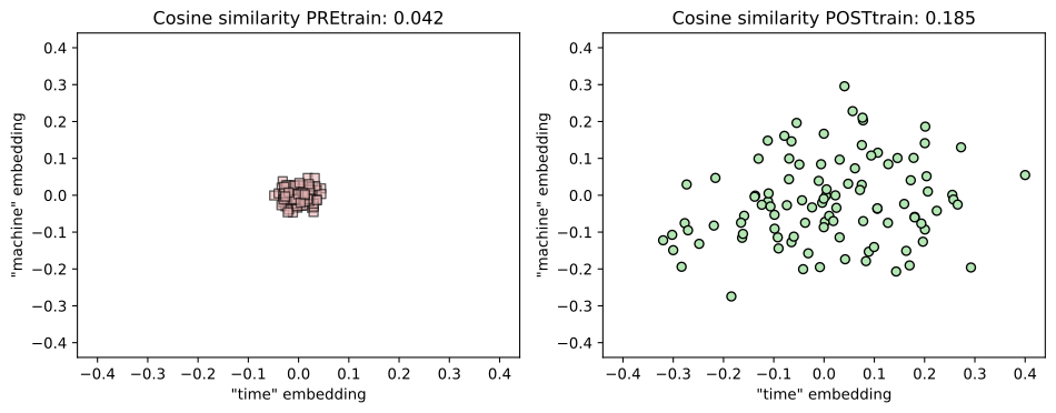
# cosine similarity manually
num = torch.dot(embed1pst,embed2pst)
den = torch.norm(embed1pst)*torch.norm(embed2pst)
cs_man = num / den

# and via pytorch
cs_pyt = F.cosine_similarity(embed2pst.unsqueeze(dim=0),embed1pst.view(1,-1))

print(f'Cosine similarity from numpy: {cs_man:.4f}')
print(f'Cosine similarity from torch: {cs_pyt.item():.4f}')Cosine similarity from numpy: 0.1854
Cosine similarity from torch: 0.1854Code below is for video "CodeChallenge: How stable are embeddings?"
Exercise 1: New training, different weights
# number of repetitions (new models) and epochs
numRepetitions = 10
numEpochs = 16

# initializations
lossesMatrix = np.zeros((numRepetitions,numEpochs))
embeddingsMats = []

# loop over repetitions
for repi in range(numRepetitions):

  # create a new model
  model = EmbeddingModel(vocab_size=nVocab, embedding_dim=embeddingDimension, context_size=context_length)
  model = model.to(device)
  for param in model.parameters():
    if param.dim()>1: nn.init.xavier_normal_(param)

  # need to recreate the optimizer b/c it retains gradient/overhead info
  optimizer = torch.optim.AdamW(model.parameters(), lr=.001, weight_decay=.01)

  # train the model
  print(f'** Running repetition {repi+1}/{numRepetitions} **')
  model,total_loss = trainTheModel(model,numEpochs)
  print('\n')

  # get its losses
  lossesMatrix[repi,:] = total_loss

  # extract the embedding matrix
embeddingsMats.append( model.embeddings.weight.detach().cpu() )** Running repetition 1/10 **
Finished epoch 1 with loss 0.2167
Finished epoch 2 with loss 0.1875
Finished epoch 3 with loss 0.1746
Finished epoch 4 with loss 0.1632183 more lines
  Finished epoch 5 with loss 0.1528
  Finished epoch 6 with loss 0.1419
  Finished epoch 7 with loss 0.1297
  Finished epoch 8 with loss 0.1157
  Finished epoch 9 with loss 0.1001
  Finished epoch 10 with loss 0.0824
  Finished epoch 11 with loss 0.0632
  Finished epoch 12 with loss 0.0436
  Finished epoch 13 with loss 0.0266
  Finished epoch 14 with loss 0.0147
  Finished epoch 15 with loss 0.0078
  Finished epoch 16 with loss 0.0042


** Running repetition 2/10 **
  Finished epoch 1 with loss 0.2169
  Finished epoch 2 with loss 0.1873
  Finished epoch 3 with loss 0.1746
  Finished epoch 4 with loss 0.1640
  Finished epoch 5 with loss 0.1539
  Finished epoch 6 with loss 0.1430
  Finished epoch 7 with loss 0.1313
  Finished epoch 8 with loss 0.1181
  Finished epoch 9 with loss 0.1030
  Finished epoch 10 with loss 0.0864
  Finished epoch 11 with loss 0.0683
  Finished epoch 12 with loss 0.0494
  Finished epoch 13 with loss 0.0318
  Finished epoch 14 with loss 0.0184
  Finished epoch 15 with loss 0.0099
  Finished epoch 16 with loss 0.0052


** Running repetition 3/10 **
  Finished epoch 1 with loss 0.2167
  Finished epoch 2 with loss 0.1881
  Finished epoch 3 with loss 0.1755
  Finished epoch 4 with loss 0.1644
  Finished epoch 5 with loss 0.1541
  Finished epoch 6 with loss 0.1433
  Finished epoch 7 with loss 0.1314
  Finished epoch 8 with loss 0.1184
  Finished epoch 9 with loss 0.1036
  Finished epoch 10 with loss 0.0876
  Finished epoch 11 with loss 0.0697
  Finished epoch 12 with loss 0.0508
  Finished epoch 13 with loss 0.0327
  Finished epoch 14 with loss 0.0186
  Finished epoch 15 with loss 0.0097
  Finished epoch 16 with loss 0.0049


** Running repetition 4/10 **
  Finished epoch 1 with loss 0.2173
  Finished epoch 2 with loss 0.1879
  Finished epoch 3 with loss 0.1757
  Finished epoch 4 with loss 0.1653
  Finished epoch 5 with loss 0.1549
  Finished epoch 6 with loss 0.1434
  Finished epoch 7 with loss 0.1305
  Finished epoch 8 with loss 0.1159
  Finished epoch 9 with loss 0.0996
  Finished epoch 10 with loss 0.0813
  Finished epoch 11 with loss 0.0614
  Finished epoch 12 with loss 0.0413
  Finished epoch 13 with loss 0.0244
  Finished epoch 14 with loss 0.0130
  Finished epoch 15 with loss 0.0065
  Finished epoch 16 with loss 0.0033


** Running repetition 5/10 **
  Finished epoch 1 with loss 0.2169
  Finished epoch 2 with loss 0.1881
  Finished epoch 3 with loss 0.1757
  Finished epoch 4 with loss 0.1650
  Finished epoch 5 with loss 0.1546
  Finished epoch 6 with loss 0.1435
  Finished epoch 7 with loss 0.1310
  Finished epoch 8 with loss 0.1171
  Finished epoch 9 with loss 0.1015
  Finished epoch 10 with loss 0.0843
  Finished epoch 11 with loss 0.0655
  Finished epoch 12 with loss 0.0462
  Finished epoch 13 with loss 0.0286
  Finished epoch 14 with loss 0.0158
  Finished epoch 15 with loss 0.0081
  Finished epoch 16 with loss 0.0043


** Running repetition 6/10 **
  Finished epoch 1 with loss 0.2173
  Finished epoch 2 with loss 0.1877
  Finished epoch 3 with loss 0.1749
  Finished epoch 4 with loss 0.1645
  Finished epoch 5 with loss 0.1541
  Finished epoch 6 with loss 0.1431
  Finished epoch 7 with loss 0.1309
  Finished epoch 8 with loss 0.1172
  Finished epoch 9 with loss 0.1021
  Finished epoch 10 with loss 0.0853
  Finished epoch 11 with loss 0.0669
  Finished epoch 12 with loss 0.0480
  Finished epoch 13 with loss 0.0309
  Finished epoch 14 with loss 0.0179
  Finished epoch 15 with loss 0.0100
  Finished epoch 16 with loss 0.0054


** Running repetition 7/10 **
  Finished epoch 1 with loss 0.2162
  Finished epoch 2 with loss 0.1874
  Finished epoch 3 with loss 0.1743
  Finished epoch 4 with loss 0.1636
  Finished epoch 5 with loss 0.1538
  Finished epoch 6 with loss 0.1434
  Finished epoch 7 with loss 0.1318
  Finished epoch 8 with loss 0.1183
  Finished epoch 9 with loss 0.1030
  Finished epoch 10 with loss 0.0856
  Finished epoch 11 with loss 0.0668
  Finished epoch 12 with loss 0.0473
  Finished epoch 13 with loss 0.0299
  Finished epoch 14 with loss 0.0167
  Finished epoch 15 with loss 0.0087
  Finished epoch 16 with loss 0.0045


** Running repetition 8/10 **
  Finished epoch 1 with loss 0.2172
  Finished epoch 2 with loss 0.1880
  Finished epoch 3 with loss 0.1756
  Finished epoch 4 with loss 0.1648
  Finished epoch 5 with loss 0.1542
  Finished epoch 6 with loss 0.1429
  Finished epoch 7 with loss 0.1303
  Finished epoch 8 with loss 0.1161
  Finished epoch 9 with loss 0.1004
  Finished epoch 10 with loss 0.0827
  Finished epoch 11 with loss 0.0635
  Finished epoch 12 with loss 0.0439
  Finished epoch 13 with loss 0.0265
  Finished epoch 14 with loss 0.0143
  Finished epoch 15 with loss 0.0073
  Finished epoch 16 with loss 0.0037


** Running repetition 9/10 **
  Finished epoch 1 with loss 0.2175
  Finished epoch 2 with loss 0.1882
  Finished epoch 3 with loss 0.1757
  Finished epoch 4 with loss 0.1644
  Finished epoch 5 with loss 0.1532
  Finished epoch 6 with loss 0.1414
  Finished epoch 7 with loss 0.1284
  Finished epoch 8 with loss 0.1138
  Finished epoch 9 with loss 0.0973
  Finished epoch 10 with loss 0.0789
  Finished epoch 11 with loss 0.0593
  Finished epoch 12 with loss 0.0400
  Finished epoch 13 with loss 0.0241
  Finished epoch 14 with loss 0.0133
  Finished epoch 15 with loss 0.0072
  Finished epoch 16 with loss 0.0040


** Running repetition 10/10 **
  Finished epoch 1 with loss 0.2163
  Finished epoch 2 with loss 0.1878
  Finished epoch 3 with loss 0.1750
  Finished epoch 4 with loss 0.1644
  Finished epoch 5 with loss 0.1541
  Finished epoch 6 with loss 0.1429
  Finished epoch 7 with loss 0.1305
  Finished epoch 8 with loss 0.1161
  Finished epoch 9 with loss 0.0997
  Finished epoch 10 with loss 0.0812
  Finished epoch 11 with loss 0.0609
  Finished epoch 12 with loss 0.0405
  Finished epoch 13 with loss 0.0232
  Finished epoch 14 with loss 0.0117
  Finished epoch 15 with loss 0.0057
Finished epoch 16 with loss 0.0030# plot the losses
plt.figure(figsize=(10,4))
# in a for-loop to get different colors
for i in range(numRepetitions):
plt.plot(lossesMatrix[i,:],'s-',linewidth=2,color=mpl.cm.plasma(i/numRepetitions),label=f'Rep. {i+1}')
plt.legend()
plt.gca().set(xticks=range(numEpochs),xlabel='Training epochs',ylabel='Losses')
plt.show()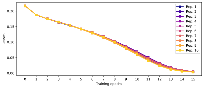
Exercise 2: Consistency of embedding vectors
_,axs = plt.subplots(3,2,figsize=(14,8))

# random words
randWords = np.random.choice(vocab,size=np.prod(axs.shape))

# but what do individual embeddings look like?
for wordi,ax in enumerate(axs.flatten()):

  # index of this random word
  randWord_idx = word2idx[randWords[wordi]]

  # loop over the repetitions
  for repi in range(numRepetitions):

    # draw lines for embeddings in each repetition
    ax.plot(embeddingsMats[repi][randWord_idx,:])

  # title of this subplot
  ax.set_title(f'"{randWords[wordi]}" embedding',fontsize=14)


# final adjustments
for a in axs.flatten(): a.set(xticks=[],yticks=[],xlim=[-1,embeddingDimension])
ax.set(xlabel='Embedding dimension',ylabel='Weight value')

plt.tight_layout()
plt.show()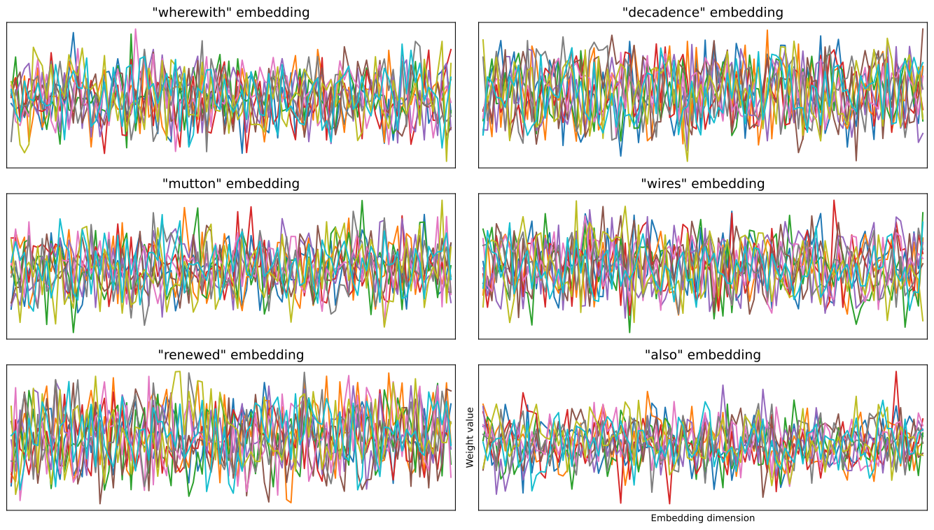
Exercise 3: Cosine similarity for selected word pairs
11. Cosine Similarity for Word Pairs
Finally, we'll examine how the semantic relationships between specific words (like "time" and "machine") evolve across multiple training repetitions.
# pick three words
word1 = 'time'
word2 = 'machine'
word3 = 'she'

# vector of cosine similarity for each repetition
cossim = np.zeros((numRepetitions,3))

# and the for-loop!
for repi in range(numRepetitions):

  # their embeddings
  e1 = embeddingsMats[repi][word2idx[word1],:]
  e2 = embeddingsMats[repi][word2idx[word2],:]
  e3 = embeddingsMats[repi][word2idx[word3],:]

  # cosine similarity between each pair
  cossim[repi,0] = nn.functional.cosine_similarity(e1,e2.view(1,-1)).item()
  cossim[repi,1] = nn.functional.cosine_similarity(e1,e3.view(1,-1)).item()
  cossim[repi,2] = nn.functional.cosine_similarity(e2,e3.view(1,-1)).item()


# the plot
plt.figure(figsize=(10,4))
plt.plot(cossim[:,0],'ks',markerfacecolor=[.9,.7,.7],markersize=12,label=f'"{word1}" and "{word2}"')
plt.plot(cossim[:,1],'ko',markerfacecolor=[.7,.8,.7],markersize=12,label=f'"{word1}" and "{word3}"')
plt.plot(cossim[:,2],'k^',markerfacecolor=[.7,.7,.8],markersize=12,label=f'"{word2}" and "{word3}"')

plt.axhline(0,color=[.7,.7,.7],linestyle='--',zorder=-10)
plt.gca().set(xticks=range(numRepetitions),ylim=[-.4,.6],
              xlabel='Training repetition',ylabel='Cosine similarity',title='Cosine similarities')
plt.legend()

plt.show()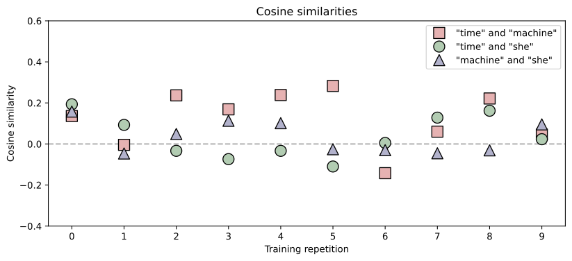
Key Take-home Points
- Data Pipeline: Building a training loop starts with text cleaning, vocabulary creation, and sequence generation for supervised learning.
- Embedding Learning: Unlike static models (GloVe), modern transformers learn embeddings from scratch as part of the total model optimization.
- Dimensionality Choice: The number of embedding dimensions is a critical hyperparameter, often balanced between representational power and computational cost.
- Semantic Evolution: As training progresses, the model pushes semantically related words closer together in the vector space, as seen in the increasing cosine similarity of related word pairs.