Adapted from A deep understanding of AI language model mechanisms — https://udemy.com/course/dullms_x
1. Setup and Environment
We'll start by importing the core PyTorch modules and our visualization tools. We'll specifically use nn.NLLLoss for calculating gradients.
import torch
import torch.nn as nn
import torch.nn.functional as F

import numpy as np
import matplotlib.pyplot as plt

import matplotlib_inline.backend_inline
matplotlib_inline.backend_inline.set_matplotlib_formats('svg')
2. Visualizing Log-Loss
Why do we use logs for loss functions? Visualizing the log curve helps us understand how the model penalizes confident but incorrect predictions compared to uncertain ones.
# the figure in the slides
p = np.linspace(.0000001,.9,500)

plt.figure(figsize=(8,3))
plt.plot(p,p,label='p',linewidth=2)
plt.plot(p,np.log(p),label='log(p)',linewidth=2)
plt.gca().set(xlabel='Probability',ylabel='Loss value',xlim=[0,p[-1]])

plt.legend(fontsize=13)
plt.show()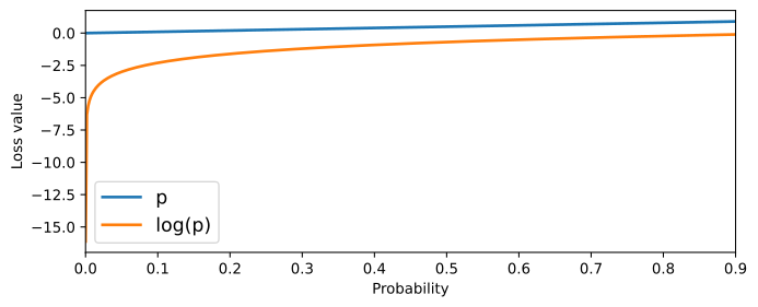
3. Negative Log-Likelihood Loss (NLLLoss)
PyTorch's NLLLoss is commonly used for classification. It expects the model to output log-probabilities, typically produced by a LogSoftmax layer.
# create a loss function instance
loss_function = nn.NLLLoss()
dir(loss_function)['T_destination',
'__annotations__',
'__call__',
'__class__',
'__constants__',116 more lines
 '__delattr__',
 '__dict__',
 '__dir__',
 '__doc__',
 '__eq__',
 '__format__',
 '__ge__',
 '__getattr__',
 '__getattribute__',
 '__getstate__',
 '__gt__',
 '__hash__',
 '__init__',
 '__init_subclass__',
 '__le__',
 '__lt__',
 '__module__',
 '__ne__',
 '__new__',
 '__reduce__',
 '__reduce_ex__',
 '__repr__',
 '__setattr__',
 '__setstate__',
 '__sizeof__',
 '__str__',
 '__subclasshook__',
 '__weakref__',
 '_apply',
 '_backward_hooks',
 '_backward_pre_hooks',
 '_buffers',
 '_call_impl',
 '_compiled_call_impl',
 '_forward_hooks',
 '_forward_hooks_always_called',
 '_forward_hooks_with_kwargs',
 '_forward_pre_hooks',
 '_forward_pre_hooks_with_kwargs',
 '_get_backward_hooks',
 '_get_backward_pre_hooks',
 '_get_name',
 '_is_full_backward_hook',
 '_load_from_state_dict',
 '_load_state_dict_post_hooks',
 '_load_state_dict_pre_hooks',
 '_maybe_warn_non_full_backward_hook',
 '_modules',
 '_named_members',
 '_non_persistent_buffers_set',
 '_parameters',
 '_register_load_state_dict_pre_hook',
 '_register_state_dict_hook',
 '_replicate_for_data_parallel',
 '_save_to_state_dict',
 '_slow_forward',
 '_state_dict_hooks',
 '_state_dict_pre_hooks',
 '_version',
 '_wrapped_call_impl',
 'add_module',
 'apply',
 'bfloat16',
 'buffers',
 'call_super_init',
 'children',
 'compile',
 'cpu',
 'cuda',
 'double',
 'dump_patches',
 'eval',
 'extra_repr',
 'float',
 'forward',
 'get_buffer',
 'get_extra_state',
 'get_parameter',
 'get_submodule',
 'half',
 'ignore_index',
 'ipu',
 'load_state_dict',
 'modules',
 'mtia',
 'named_buffers',
 'named_children',
 'named_modules',
 'named_parameters',
 'parameters',
 'reduction',
 'register_backward_hook',
 'register_buffer',
 'register_forward_hook',
 'register_forward_pre_hook',
 'register_full_backward_hook',
 'register_full_backward_pre_hook',
 'register_load_state_dict_post_hook',
 'register_load_state_dict_pre_hook',
 'register_module',
 'register_parameter',
 'register_state_dict_post_hook',
 'register_state_dict_pre_hook',
 'requires_grad_',
 'set_extra_state',
 'set_submodule',
 'share_memory',
 'state_dict',
 'to',
 'to_empty',
 'train',
 'training',
 'type',
 'weight',
 'xpu',
 'zero_grad']
Understanding Log-Softmax Inputs
Let's trace how a raw model output (logits) is transformed into log-softmax values and then used to calculate the loss for different target categories.
# start with three outputs (raw model outputs for three tokens in the vocab)
model_output = torch.tensor([[ -1, 2.3, .1 ]], dtype=torch.float64, requires_grad=True)
print('Raw model outputs:')
print(f'  {model_output[0].tolist()}\n')

# NLLLoss expects log-softmax inputs!
logsoftmax_output = F.log_softmax(model_output,dim=-1)
print('Log-softmax model outputs:')
print('  ',[round(o.item(),2) for o in logsoftmax_output[0] ],'\n')


# check the loss for different targets
for target in range(len(model_output[0])):

  # which output is the target (correct response)?
  target = torch.tensor([target])

  # calculate the loss
  theloss = loss_function(logsoftmax_output,target)

  # and print
print(f'When the correct output is index "{target.item()}", the loss is {theloss.item():.2f}')Raw model outputs:
[-1.0, 2.3, 0.1]
Log-softmax model outputs:
[-3.44, -0.14, -2.34] 4 more lines
When the correct output is index "0", the loss is 3.44
When the correct output is index "1", the loss is 0.14
When the correct output is index "2", the loss is 2.34
4. Batch Loss Processing
In practice, we process multiple samples simultaneously in a batch. NLLLoss calculates the average loss across all samples in the batch.
# let's create four batches
batch_output = model_output.repeat(4,1)
print(batch_output,'\n')

# but of course we need logsoftmax
logsoftmax_output = F.log_softmax(batch_output,dim=1)
print(logsoftmax_output)tensor([[-1.0000, 2.3000, 0.1000],
[-1.0000, 2.3000, 0.1000],
[-1.0000, 2.3000, 0.1000],
[-1.0000, 2.3000, 0.1000]], dtype=torch.float64,
grad_fn=<RepeatBackward0>) 6 more lines
tensor([[-3.4377, -0.1377, -2.3377],
        [-3.4377, -0.1377, -2.3377],
        [-3.4377, -0.1377, -2.3377],
        [-3.4377, -0.1377, -2.3377]], dtype=torch.float64,
       grad_fn=<LogSoftmaxBackward0>)
Batch Optimization Logic
We'll define a set of targets for our batch and calculate the aggregate loss, which can then be used to update the model's weights via backpropagation.
# target changes for each batch
targets = torch.tensor([0,1,2,0])loss = loss_function(logsoftmax_output,targets)
print(loss)tensor(2.3377, dtype=torch.float64, grad_fn=<NllLossBackward0>)# again, manual calculation
-torch.tensor([ -3.4377 + -0.1377 + -2.3377 + -3.4377 ]) / len(targets)tensor([2.3377])loss.backward()5. Simple PyTorch Optimization Loop
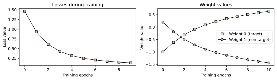
Now we'll put it all together. We'll create a single weight vector and use Stochastic Gradient Descent (SGD) to minimize the loss for a specific target token.
# define a weight matrix (requires_grad=True to track gradients)
w = torch.tensor([[-1,.2]], requires_grad=True)

# target category
target = torch.tensor([0])

# optimizer
optimizer = torch.optim.SGD([w],lr=.5)

# training iterations
numTrainingIters = 10

# initialize some variables
allWeights = torch.zeros((numTrainingIters+1,2))
allWeights[0,:] = w.detach()
allLosses = torch.zeros(numTrainingIters)

# training loop
for i in range(numTrainingIters):

  # reset gradients
  optimizer.zero_grad()

  # model outputs (simulating a full model forward pass ;)  )
  modeloutput = F.log_softmax(w,dim=1)

  # loss
  loss = loss_function(modeloutput,target)
  allLosses[i] = loss.item()

  # gradient descent
  loss.backward()  # calculate gradient of loss wrt w
  optimizer.step() # adjust w using SGD

  # store the new weights
  allWeights[i+1,:] = w.detach()

  # and print out some results
print(f"Step {i+1:2d}: loss = {loss.item():.3f}, weights = {[round(o.item(),2) for o in w[0] ]}")Step 1: loss = 1.463, weights = [-0.62, -0.18]
Step 2: loss = 0.932, weights = [-0.31, -0.49]
Step 3: loss = 0.610, weights = [-0.08, -0.72]
Step 4: loss = 0.427, weights = [0.09, -0.89]
Step 5: loss = 0.319, weights = [0.23, -1.03]5 more lines
Step  6: loss = 0.252, weights = [0.34, -1.14]
Step  7: loss = 0.206, weights = [0.43, -1.23]
Step  8: loss = 0.174, weights = [0.51, -1.31]
Step  9: loss = 0.150, weights = [0.58, -1.38]
Step 10: loss = 0.132, weights = [0.64, -1.44]
6. Training Results Visualization
By plotting the loss and weight values over time, we can observe the model "learning" as the target weight increases and the loss converges toward zero.
# let's see the weights!
_,axs = plt.subplots(1,2,figsize=(10,3))


axs[0].plot(allLosses,'ks-',linewidth=1,markerfacecolor=[.9,.7,.7])
axs[0].set(xlabel='Training epochs',ylabel='Loss value',title='Losses during training')

axs[1].plot(allWeights[:,0],'ks-',markerfacecolor=[.7,.9,.7],linewidth=1,label='Weight 0 (target)')
axs[1].plot(allWeights[:,1],'ko-',markerfacecolor=[.7,.7,.9],linewidth=1,label='Weight 1 (non-target)')
axs[1].set(xlabel='Training epochs',ylabel='Weight value',title='Weight values')
axs[1].legend()

plt.tight_layout()
plt.show()
Key Take-home Points
- Logarithmic Scaling: Using log-probabilities for loss functions provides a steeper gradient when the model is very wrong, accelerating learning.
- LogSoftmax and NLLLoss: In PyTorch, the combination of
nn.LogSoftmaxandnn.NLLLossis the standard way to implement Cross Entropy for classification. - Average Batch Loss: Losses are typically calculated as the mean across an entire batch, ensuring stable gradient updates regardless of batch size.
- Weight Convergence: During training, the weights associated with the correct target are pushed higher while others are suppressed, minimizing the total loss.