7. The Unembedding Layer | Driptanil Datta

Adapted from A deep understanding of AI language model mechanisms — https://udemy.com/course/dullms_x

The Lifecycle of a Token

Before diving into the code, let's look at where the unembedding layer fits in the LLM architecture.

Text is converted into tokens, but LLMs work with embeddings.
Tokens must be converted into embeddings before the LLM.
LLMs modify the embeddings (via Attention) for classification and generation.
The unembeddings matrix transforms embedding vectors back into token integers.

python

import numpy as np
import matplotlib.pyplot as plt

import matplotlib_inline.backend_inline
matplotlib_inline.backend_inline.set_matplotlib_formats('svg')

from transformers import GPT2Model,GPT2Tokenizer

# pretrained GPT-2 model and tokenizer
gpt2 = GPT2Model.from_pretrained('gpt2')
tokenizer = GPT2Tokenizer.from_pretrained('gpt2')

Weight Extraction

We isolate the word token embedding (WTE) weights from the model to use as our base for the unembedding layer.

python

# embeddings matrix
embeddings = gpt2.wte.weight.detach().numpy()

python

# find the size parameters in .config
gpt2.config

Out · result

GPT2Config {
  "_attn_implementation_autoset": true,
  "activation_function": "gelu_new",
  "architectures": [
    "GPT2LMHeadModel"

34 more lines

  ],
  "attn_pdrop": 0.1,
  "bos_token_id": 50256,
  "embd_pdrop": 0.1,
  "eos_token_id": 50256,
  "initializer_range": 0.02,
  "layer_norm_epsilon": 1e-05,
  "model_type": "gpt2",
  "n_ctx": 1024,
  "n_embd": 768,
  "n_head": 12,
  "n_inner": null,
  "n_layer": 12,
  "n_positions": 1024,
  "reorder_and_upcast_attn": false,
  "resid_pdrop": 0.1,
  "scale_attn_by_inverse_layer_idx": false,
  "scale_attn_weights": true,
  "summary_activation": null,
  "summary_first_dropout": 0.1,
  "summary_proj_to_labels": true,
  "summary_type": "cls_index",
  "summary_use_proj": true,
  "task_specific_params": {
    "text-generation": {
      "do_sample": true,
      "max_length": 50
    }
  },
  "torch_dtype": "float32",
  "transformers_version": "4.51.3",
  "use_cache": true,
  "vocab_size": 50257
}

python

# the properties we'll use later
print(f'Embedding dimensions: {gpt2.config.n_embd}')
print(f'Vocab size: {gpt2.config.vocab_size}')
print(f'Size of embeddings matrix: {embeddings.shape}')

Out · stdout

Embedding dimensions: 768
Vocab size: 50257
Size of embeddings matrix: (50257, 768)

3. Real vs. Random Unembeddings

Before we look at the code, it's worth asking: Where do unembeddings matrices come from? There are two primary strategies used in modern LLMs:

Feature	Trained Unembeddings	"Tied" Unembeddings
Origin	Initialized as random numbers and optimized through gradient descent.	A transposed copy of the existing embeddings matrix.
Efficiency	Specifically optimized for output performance.	No additional training or parameters required.
Trade-offs	Adds a large number of parameters to train with often unclear benefits.	The transformed embedding space might differ from the initial space.

Why Transpose? (Weight Tying)

In many modern architectures (including GPT-2), the unembedding matrix is simply the transpose of the embedding matrix. This technique is known as Weight Tying.

The intuition is simple: if a specific vector represents the concept of "Apple" when the model reads it, that same vector should be what the model produces when it wants to say "Apple."

Mathematically, when we use the transpose, the score (logit) for a token $i$ is calculated as: $\text{score}_i = \vec{h} \cdot \vec{e}_i$ Where:

$\vec{h}$ is the model's final hidden state (its "thought").
$\vec{e}_i$ is the embedding vector for token $i$ .

The model is essentially performing a similarity search across its entire vocabulary, looking for the embedding that most closely matches its current internal state.

python

# unembeddings matrix as the transpose of the (real) embeddings
unembeddings = embeddings.T

# confirm that transposing matrix a copy
print('id of embeddings:  ',id(embeddings))
print('id of unembeddings:',id(unembeddings))

Out · stdout

id of embeddings:   4513828656
id of unembeddings: 4964714512

python

# a random unembeddings matrix
unembeddingsRand = np.random.randn(gpt2.config.n_embd,gpt2.config.vocab_size)

print(f'         Size of embeddings matrix: {embeddings.shape}')
print(f'Size of random unembeddings matrix: {unembeddingsRand.shape}')
print(f'  Size of real unembeddings matrix: {unembeddings.shape}')

Out · stdout

         Size of embeddings matrix: (50257, 768)
Size of random unembeddings matrix: (768, 50257)
  Size of real unembeddings matrix: (768, 50257)

4. Visualizing a Specific Embedding

Let's pick a specific word, "California," and visualize its embedding vector. This 768-dimensional signature is what the model uses to represent the concept.

python

# pick a word
seedword = ' California'

# its token index
seed_idx = tokenizer.encode(seedword)

# make sure it's one token
seed_idx

Out · result

[3442]

python

# find its embedding vector
embed_vector = embeddings[seed_idx,:]

# plot it!
plt.figure(figsize=(10,3))
plt.scatter(range(gpt2.config.n_embd),embed_vector.squeeze(),s=30,c=abs(embed_vector),cmap='RdPu')
plt.gca().set(xlabel='Embedding dimension',ylabel='Embedding weight',xlim=[-3,gpt2.config.n_embd+2],
              title=f'Embedding (GPT2) of "{tokenizer.decode(seed_idx)}"')
plt.show()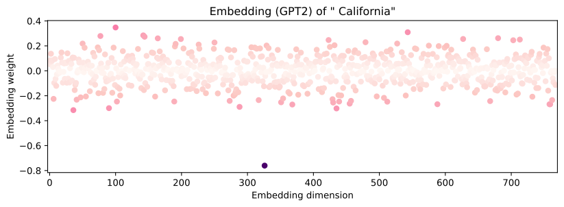

Mapping Back to Tokens

By projecting our vector onto the unembedding matrices (via a dot product), we can see which tokens the model thinks are most similar to our seed concept.

python

# project the embedding vector onto the unembedding matrix
dpRand = embed_vector @ unembeddingsRand

# next token is the maximum dot product (unscaled cosine similarity)!
nextTokenRand_idx = np.argmax(dpRand)
nextTokenRand = tokenizer.decode(nextTokenRand_idx)

# check the sizes
print('embed_vector  X  unembeddings  =  dotproducts')
print(f'  {embed_vector.shape}       {unembeddingsRand.shape}      {dpRand.shape}')

Out · stdout

embed_vector  X  unembeddings  =  dotproducts
  (1, 768)       (768, 50257)      (1, 50257)

python

# repeat for the real unembeddings matrix
dpReal = embed_vector @ unembeddings
nextTokenReal_idx = np.argmax(dpReal)
nextTokenReal = tokenizer.decode(nextTokenReal_idx)

python

print('** Random unembeddings matrix:')
print(f'   "{tokenizer.decode(seed_idx)}" has largest dot product with token "{nextTokenRand}"\n')

print('** Real unembeddings matrix:')
print(f'   "{tokenizer.decode(seed_idx)}" has largest dot product with token "{nextTokenReal}"')

Out · stdout

** Random unembeddings matrix:
   " California" has largest dot product with token " hurting"

** Real unembeddings matrix:
" California" has largest dot product with token "California"

Distribution Comparison

Plotting the dot products across the entire vocabulary reveals how the real unembedding matrix effectively "identifies" the original token, while the random matrix produces noise.

python

# plot it!
_,axs = plt.subplots(1,2,figsize=(12,3))
axs[0].scatter(range(tokenizer.vocab_size),dpRand,s=30,c=abs(dpRand),cmap='RdPu',alpha=.4)
axs[0].axvline(nextTokenRand_idx,linestyle='--',color='k',alpha=1/3)
axs[0].plot(nextTokenRand_idx,dpRand[0,nextTokenRand_idx],'gv')
axs[0].set(xlabel='Unembedding dimension',ylabel='Dot product',xlim=[-11,tokenizer.vocab_size+10],
              title=f'(Random) dot products with "{tokenizer.decode(seed_idx)}"')

axs[1].scatter(range(tokenizer.vocab_size),dpReal,s=30,c=abs(dpReal),cmap='RdPu',alpha=.4)
axs[1].axvline(nextTokenReal_idx,linestyle='--',color='k',alpha=1/3)
axs[1].plot(nextTokenReal_idx,dpReal[0,nextTokenReal_idx],'gv')
axs[1].set(xlabel='Unembedding dimension',ylabel='Dot product',xlim=[-11,tokenizer.vocab_size+10],
              title=f'(Real) dot products with "{tokenizer.decode(seed_idx)}"')


plt.tight_layout()
plt.show()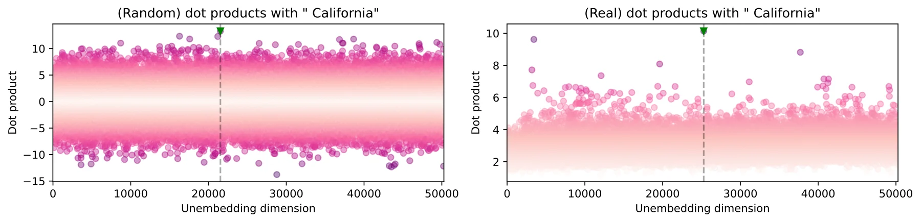

5. Analyzing Top-10 Projections

Beyond the identical token, what other words are "close" to California in the embedding space? We'll examine the top 10 results from the real unembedding matrix.

python

top10 = np.argsort(dpReal[0])[::-1][:10]

for i in top10:
  print(f'Dot product {dpReal[0,i]:6.3f} for token "{tokenizer.decode(i)}"')

Out · stdout

Dot product 10.136 for token "California"
Dot product  9.617 for token " California"
Dot product  8.816 for token " Californ"
Dot product  8.088 for token "Calif"
Dot product  7.718 for token " Calif"

5 more lines

Dot product  7.359 for token " Nevada"
Dot product  7.158 for token "Arizona"
Dot product  7.151 for token "Colorado"
Dot product  6.974 for token "Florida"
Dot product  6.912 for token "Oregon"

6. Generative Sequence Experiment

We can use our unembedding logic to "generate" a sequence of text by iteratively picking tokens that are semantically close to the previous one.

python

# sequence length
seq_len = 10

# initial seed
nextword = 'budget'

# initializing a list that will contain the text
text = nextword


# loop to create the sequence
for i in range(seq_len-1):

  # step 1: tokenize
  token = tokenizer.encode(nextword)

  # step 2: get embedding vector
  embed_vector = embeddings[token,:]

  # step 3: project onto unembedding matrix (dot products)
  dp = embed_vector @ unembeddings

  # step 4: find top10 projections
  top10 = np.argsort(dp[0])[::-1][:10]

  # step 5: randomly pick one for next token
  aRandomToken = np.random.choice(top10)
  nextword = tokenizer.decode(aRandomToken)

  # step 6: append the text
  text += nextword

# print the final result!
print('Our very philosophically meaningful text:\n',text)

Out · stdout

Our very philosophically meaningful text:
 budget contrace sacrific sacrific advoc corrid mathemat challeng conclud conduc

7. Comparing with Random Noise

Finally, we repeat the generation process using the random unembedding matrix to see how meaningful semantic relationships are lost when the mapping layer is untrained.

python

# initialize
nextword = 'budget'
text = nextword

# loop
for i in range(seq_len-1):

  # step 1: tokenize
  token = tokenizer.encode(nextword)

  # step 2: get embedding vector
  embed_vector = embeddings[token,:]

  # step 3: project onto RANDOM unembedding matrix
  dp = embed_vector @ unembeddingsRand

  # step 4: find top10 projections
  top10 = np.argsort(dp[0])[::-1][:10]

  # step 5: randomly pick one for next token
  aRandomToken = np.random.choice(top10)
  nextword = tokenizer.decode(aRandomToken)

  # step 6: append the text
  text += nextword

print('Our randomly meanderingful text:\n',text)

Key Take-home Points

Conceptual Inverse: An "unembeddings matrix" is the conceptual inverse of the embeddings matrix (but not a literal inverse matrix).
Simplicity: The broad strokes mechanisms of next-token generation is simple conceptually and mathematically.
Top Token: The token with the largest unembeddings value is the next token in a generated sequence.
Semantic Drift: Generated text can quickly lose meaning, which was a major hurdle for language models to overcome.

Out · stdout

Our randomly meanderingful text:
 budget Happ Barrellow Arkansas threatens syndromeifer Asian organism