Adapted from A deep understanding of AI language model mechanisms — https://udemy.com/course/dullms_x
1. Environment Setup
We'll begin by importing our visualization tools and configuring the plotting backend for high-quality SVG outputs.
import numpy as np
import matplotlib.pyplot as plt
from matplotlib.gridspec import GridSpec

# higher-res plots
import matplotlib_inline.backend_inline
matplotlib_inline.backend_inline.set_matplotlib_formats('svg')
2. Loading GPT-2 and BERT
In this lesson, we compare two foundational transformer models: GPT-2 (decoder-only) and BERT (encoder-only). We'll start by loading their respective models and tokenizers from the transformers library.
from transformers import GPT2Model,GPT2Tokenizer
gpt2 = GPT2Model.from_pretrained('gpt2')
tokenizerG = GPT2Tokenizer.from_pretrained('gpt2')/Users/drippy/.pyenv/versions/3.12.6/lib/python3.12/site-packages/tqdm/auto.py:21: TqdmWarning: IProgress not found. Please update jupyter and ipywidgets. See https://ipywidgets.readthedocs.io/en/stable/user_install.html
from .autonotebook import tqdm as notebook_tqdmfrom transformers import BertTokenizer, BertModel
tokenizerB = BertTokenizer.from_pretrained('bert-base-uncased')
bert = BertModel.from_pretrained('bert-base-uncased')3. Architecture Inspection
Let's look at the internal structure of both models. Notice the differences in their embedding layers and block architectures.
# check out the model
print(gpt2)GPT2Model(
(wte): Embedding(50257, 768)
(wpe): Embedding(1024, 768)
(drop): Dropout(p=0.1, inplace=False)
(h): ModuleList(19 more lines
    (0-11): 12 x GPT2Block(
      (ln_1): LayerNorm((768,), eps=1e-05, elementwise_affine=True)
      (attn): GPT2Attention(
        (c_attn): Conv1D(nf=2304, nx=768)
        (c_proj): Conv1D(nf=768, nx=768)
        (attn_dropout): Dropout(p=0.1, inplace=False)
        (resid_dropout): Dropout(p=0.1, inplace=False)
      )
      (ln_2): LayerNorm((768,), eps=1e-05, elementwise_affine=True)
      (mlp): GPT2MLP(
        (c_fc): Conv1D(nf=3072, nx=768)
        (c_proj): Conv1D(nf=768, nx=3072)
        (act): NewGELUActivation()
        (dropout): Dropout(p=0.1, inplace=False)
      )
    )
  )
  (ln_f): LayerNorm((768,), eps=1e-05, elementwise_affine=True)
)# check out the model
print(bert)BertModel(
(embeddings): BertEmbeddings(
(word_embeddings): Embedding(30522, 768, padding_idx=0)
(position_embeddings): Embedding(512, 768)
(token_type_embeddings): Embedding(2, 768)36 more lines
    (LayerNorm): LayerNorm((768,), eps=1e-12, elementwise_affine=True)
    (dropout): Dropout(p=0.1, inplace=False)
  )
  (encoder): BertEncoder(
    (layer): ModuleList(
      (0-11): 12 x BertLayer(
        (attention): BertAttention(
          (self): BertSdpaSelfAttention(
            (query): Linear(in_features=768, out_features=768, bias=True)
            (key): Linear(in_features=768, out_features=768, bias=True)
            (value): Linear(in_features=768, out_features=768, bias=True)
            (dropout): Dropout(p=0.1, inplace=False)
          )
          (output): BertSelfOutput(
            (dense): Linear(in_features=768, out_features=768, bias=True)
            (LayerNorm): LayerNorm((768,), eps=1e-12, elementwise_affine=True)
            (dropout): Dropout(p=0.1, inplace=False)
          )
        )
        (intermediate): BertIntermediate(
          (dense): Linear(in_features=768, out_features=3072, bias=True)
          (intermediate_act_fn): GELUActivation()
        )
        (output): BertOutput(
          (dense): Linear(in_features=3072, out_features=768, bias=True)
          (LayerNorm): LayerNorm((768,), eps=1e-12, elementwise_affine=True)
          (dropout): Dropout(p=0.1, inplace=False)
        )
      )
    )
  )
  (pooler): BertPooler(
    (dense): Linear(in_features=768, out_features=768, bias=True)
    (activation): Tanh()
  )
)
4. Vocabulary Size Comparison
GPT-2 and BERT use different tokenization strategies (Byte-Pair Encoding vs. WordPiece), which leads to different total vocabulary sizes.
print(f'BERT has {tokenizerB.vocab_size:,} tokens.')
print(f'GPT2 has {tokenizerG.vocab_size:,} tokens.')BERT has 30,522 tokens.
GPT2 has 50,257 tokens.5. Token Length Distribution
We can analyze the distribution of token lengths (in characters) to see how each model decomposes language into subword units.
# GPT: get all individual lengths
token_lengths = np.zeros(tokenizerG.vocab_size,dtype=int)
for idx,word in enumerate( tokenizerG.encoder.keys() ):
  token_lengths[idx] = len(word)

# unique values and counts for bar plot
uniqueLengthsG,tokenCountG = np.unique(token_lengths,return_counts=True)


# BERT: get all individual lengths
token_lengths = np.zeros(tokenizerB.vocab_size,dtype=int)
for idx,word in enumerate( tokenizerB.get_vocab().keys() ): # note difference from GPT!
  token_lengths[idx] = len(word)

# unique values and counts for bar plot
uniqueLengthsB,tokenCountB = np.unique(token_lengths,return_counts=True)# draw the barplot!
_,axs = plt.subplots(2,1,figsize=(8,6))
axs[0].bar(uniqueLengthsG,tokenCountG,color='k',edgecolor='gray')
axs[0].set(xlabel='Token length (chars)',ylabel='Token count',title='GPT2 token lengths (clipped at 22)',
xlim=[0,22])
axs[1].bar(uniqueLengthsB,tokenCountB,color='k',edgecolor='gray')
axs[1].set(xlabel='Token length (chars)',ylabel='Token count',title='BERT token lengths',
xlim=[0,22])
plt.tight_layout()
plt.show()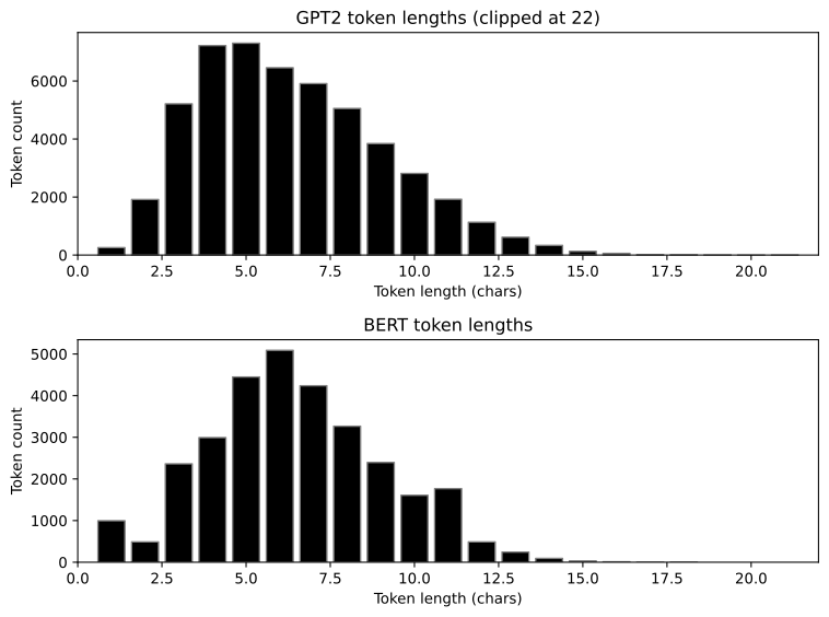
6. Embedding Matrix Extraction
We can extract the raw word token embedding matrices to analyze their weights directly as NumPy arrays.
# get the Word Token Embeddings matrix
embeddingsG = gpt2.wte.weight.detach().numpy()

# get the word token embeddings matrix (note the different variable names compared to GPT2!
embeddingsB = bert.embeddings.word_embeddings.weight.detach().numpy()

# print their sizes
print(f'BERT embedding matrix is of size {embeddingsB.shape}.')
print(f'GPT2 embedding matrix is of size {embeddingsG.shape}.')BERT embedding matrix is of size (30522, 768).
GPT2 embedding matrix is of size (50257, 768).Weight Visualization
Visualizing the full embedding matrix reveals the density and variance of weights across all dimensions and tokens.
fig,axs = plt.subplots(2,1,figsize=(10,8))

# GPT embeddings
h = axs[0].imshow(embeddingsG.T,aspect='auto',vmin=-.15,vmax=.15)
axs[0].set(xlabel='Tokens',ylabel='Dimensions',title='GPT-2 embeddings matrix')
fig.colorbar(h,ax=axs[0],pad=.01)

# BERT embeddings
h = axs[1].imshow(embeddingsB.T,aspect='auto',vmin=-.15,vmax=.15)
axs[1].set(xlabel='Tokens',ylabel='Dimensions',title='BERT embedding matrix')
fig.colorbar(h,ax=axs[1],pad=.01)

plt.tight_layout()
plt.show()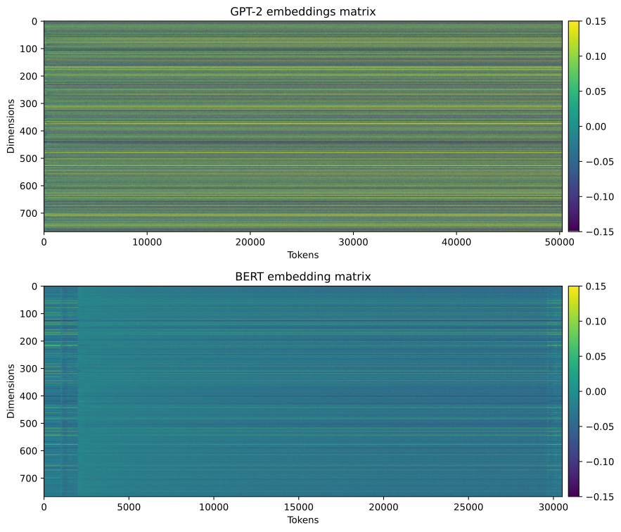
7. Direct Token Comparison
What happens if we compare the same token index across models? Since their vocabularies are sorted differently, the same index will likely represent completely different concepts.
# pick a random token index
ridx = np.random.randint(10000,20000)

_,axs = plt.subplots(1,2,figsize=(12,4))

axs[0].plot(embeddingsB[ridx,:],label='BERT',linewidth=.5)
axs[0].plot(embeddingsG[ridx,:],label='GPT2',linewidth=.5)
axs[0].legend()
axs[0].set(xlabel='Embeddings dimension',ylabel='Embedding value',xlim=[0,embeddingsB.shape[1]],title=f'Token {ridx}')

axs[1].plot(embeddingsB[ridx,:],embeddingsG[ridx,:],'s',markerfacecolor=[.7,.9,.7])
axs[1].set(xlabel=f'BERT ("{tokenizerB.decode(ridx)}")',ylabel=f'GPT2 ("{tokenizerG.decode(ridx)}")',
           title='Embedding comparison')

plt.show()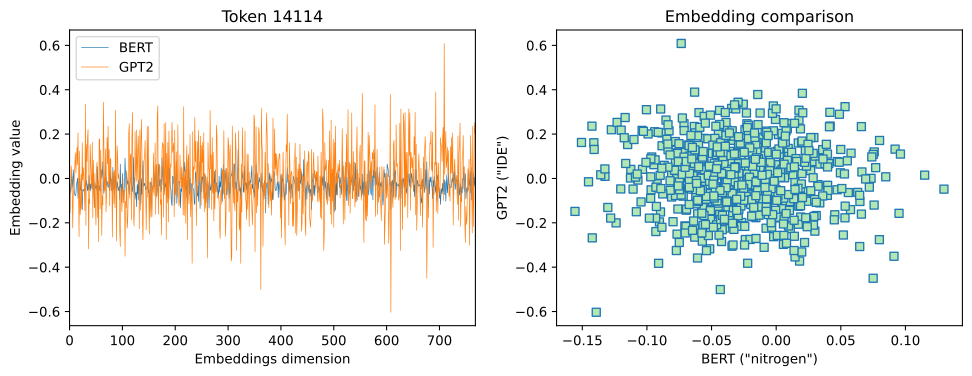
Semantic Alignment
When we look at the same word (like "the") across both models, we can check if their vector representations are correlated despite being trained independently.
# how about the same word?
token = 'the'
token_idxB = tokenizerB.encode(token)[1]
token_idxG = tokenizerG.encode(token)[0]

print(f'BERT: "{token}" is index {token_idxB}')
print(f'GPT2: "{token}" is index {token_idxG}')BERT: "the" is index 1996
GPT2: "the" is index 1169# their correlation
corr = np.corrcoef(embeddingsB[token_idxB,:],embeddingsG[token_idxG,:])
plt.plot(embeddingsB[token_idxB,:],embeddingsG[token_idxG,:],'s',markerfacecolor=[.7,.9,.9])
plt.gca().set(xlabel=f'BERT ("{tokenizerB.decode(token_idxB)}")',ylabel=f'GPT2 ("{tokenizerG.decode(token_idxG)}")',
title=f'Embedding comparison (r = {corr[0,1]:.2f})')
plt.show()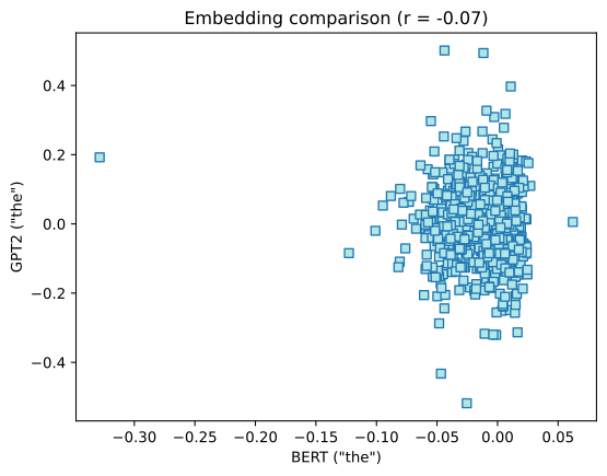
8. Statistical Properties
Finally, we analyze the global distribution of means and variances for the embedding vectors to ensure they are well-normalized.
_,axs = plt.subplots(1,2,figsize=(12,3.5))

# compare the embeddings variances
yB,xB = np.histogram(embeddingsB.var(axis=1),bins=100,density=True)
yG,xG = np.histogram(embeddingsG.var(axis=1),bins=100,density=True)

axs[0].plot(xB[:-1],yB,linewidth=2,label='BERT')
axs[0].plot(xG[:-1],yG,linewidth=2,label='GPT2')
axs[0].set(xlabel='Variance',ylabel='Density',xlim=[0,None],ylim=[0,None],title='Variances distributions')
axs[0].legend()

# compare the embeddings means
yB,xB = np.histogram(embeddingsB.mean(axis=1),bins=100,density=True)
yG,xG = np.histogram(embeddingsG.mean(axis=1),bins=100,density=True)

axs[1].plot(xB[:-1],yB,linewidth=2,label='BERT')
axs[1].plot(xG[:-1],yG,linewidth=2,label='GPT2')
axs[1].axvline(0,color=[.7,.7,.7],linestyle='--')
axs[1].set(xlabel='Average',ylabel='Density',ylim=[0,None],title='Means distributions')
axs[1].legend()


plt.show()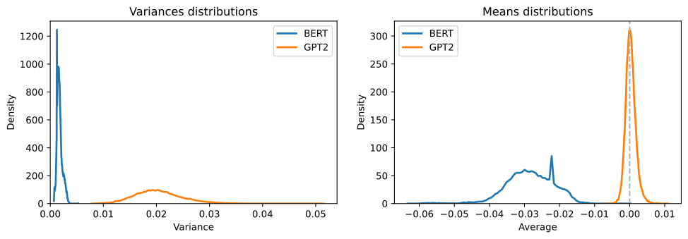
Key Take-home Points
- Different Strategies: BERT and GPT-2 use different tokenization schemes (WordPiece vs. BPE) and have different vocabulary sizes (~30k vs ~50k).
- Architectural Nuances: GPT-2's embeddings are learned for a decoder-only task, while BERT is encoder-only, leading to different weight distributions.
- Vocabulary Mismatch: A specific token index (e.g., 1000) does not map to the same word across models.
- Semantic Correlation: Even with different architectures, high-frequency words like "the" often show positive correlation in their vector spaces.