2. Wikipedia vs. Twitter | Driptanil Datta

Adapted from A deep understanding of AI language model mechanisms — https://udemy.com/course/dullms_x

1. Setup and Environment

We'll start by configuring our environment and ensuring we can render high-quality SVG plots for our comparisons.

python

import numpy as np
import matplotlib.pyplot as plt
import matplotlib as mpl

# svg figure format
import matplotlib_inline.backend_inline
matplotlib_inline.backend_inline.set_matplotlib_formats('svg')

2. Comparing GloVe Models

In this exercise, we download two distinct GloVe models: glove-wiki-gigaword-50 and glove-twitter-50. This allows us to compare how formal text (Wikipedia) and informal text (Twitter) shape word representations.

python

# NOTE: If you get errors importing, run the following !pip... line,
# then restart your session (from Runtime menu) and comment out the pip line.
# !pip install gensim

import gensim.downloader as api

# download the wikipedia and twitter models
wiki = api.load('glove-wiki-gigaword-50')
twit = api.load('glove-twitter-50')

Inspecting Model Properties

We can peek at the internal methods of the models to see how they handle their vocabularies.

python

dir(twit)

Out · result

['__class__',
 '__contains__',
 '__delattr__',
 '__dict__',
 '__dir__',

92 more lines

 '__doc__',
 '__eq__',
 '__format__',
 '__ge__',
 '__getattribute__',
 '__getitem__',
 '__getstate__',
 '__gt__',
 '__hash__',
 '__init__',
 '__init_subclass__',
 '__le__',
 '__len__',
 '__lt__',
 '__module__',
 '__ne__',
 '__new__',
 '__reduce__',
 '__reduce_ex__',
 '__repr__',
 '__setattr__',
 '__setitem__',
 '__sizeof__',
 '__str__',
 '__subclasshook__',
 '__weakref__',
 '_adapt_by_suffix',
 '_load_specials',
 '_log_evaluate_word_analogies',
 '_save_specials',
 '_smart_save',
 '_upconvert_old_d2vkv',
 '_upconvert_old_vocab',
 'add_lifecycle_event',
 'add_vector',
 'add_vectors',
 'allocate_vecattrs',
 'closer_than',
 'cosine_similarities',
 'distance',
 'distances',
 'doesnt_match',
 'evaluate_word_analogies',
 'evaluate_word_pairs',
 'expandos',
 'fill_norms',
 'get_index',
 'get_mean_vector',
 'get_normed_vectors',
 'get_vecattr',
 'get_vector',
 'has_index_for',
 'index2entity',
 'index2word',
 'index_to_key',
 'init_sims',
 'intersect_word2vec_format',
 'key_to_index',
 'lifecycle_events',
 'load',
 'load_word2vec_format',
 'log_accuracy',
 'log_evaluate_word_pairs',
 'mapfile_path',
 'most_similar',
 'most_similar_cosmul',
 'most_similar_to_given',
 'n_similarity',
 'next_index',
 'norms',
 'rank',
 'rank_by_centrality',
 'relative_cosine_similarity',
 'resize_vectors',
 'save',
 'save_word2vec_format',
 'set_vecattr',
 'similar_by_key',
 'similar_by_vector',
 'similar_by_word',
 'similarity',
 'similarity_unseen_docs',
 'sort_by_descending_frequency',
 'unit_normalize_all',
 'vector_size',
 'vectors',
 'vectors_for_all',
 'vectors_norm',
 'vocab',
 'wmdistance',
 'word_vec',
 'words_closer_than']

3. Embedding Matrix Analysis

Let's compare the vocabulary size and embedding dimensions for both models. Notice that while both use 50-dimensional vectors, their vocabularies differ significantly in size.

python

# embedding matrix dimensions
print(f'Wikipedia model has {wiki.vectors.shape[0]:,} words and {wiki.vectors.shape[1]} embedding dimensions.')
print(f'Twitter model has {twit.vectors.shape[0]:,} words and {twit.vectors.shape[1]} embedding dimensions.')

Out · stdout

Wikipedia model has 400,000 words and 50 embedding dimensions.
Twitter model has 1,193,514 words and 50 embedding dimensions.

4. Visualizing Vector Differences

To see the difference in representation, we can plot the vector for a single word (like "table") from both models and compare them directly.

python

targetword = 'table'

_,axs = plt.subplots(1,2,figsize=(12,4.5))
axs[0].plot(wiki[targetword],'ks',markerfacecolor=[.7,.7,.9],markersize=8,label='Wikipedia')
axs[0].plot(twit[targetword],'ko',markerfacecolor=[.7,.9,.7],markersize=8,label='Twitter')
axs[0].set(xlabel='Dimension',ylabel='Value',title=f'Embeddings for "{targetword}"')
axs[0].legend()

axs[1].plot(wiki[targetword],twit[targetword],'k^',markerfacecolor=[.9,.7,.7],markersize=8)
axs[1].set(xlabel='Wiki embedding',ylabel='Twitter embedding',title=f'Embeddings for "{targetword}"')

plt.tight_layout()
plt.show()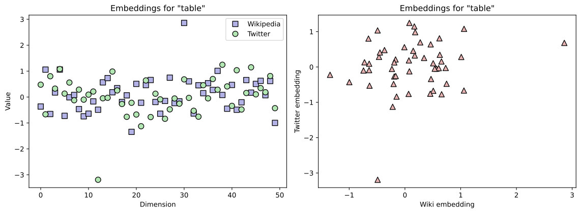

5. Pairwise Semantic Relationships

How does the semantic relationship between two words (e.g., "table" and "chair") change depending on the training data? We'll use cosine similarity to find out.

python

# word pair
word1 = 'table'
word2 = 'chair'

# scatter plot for wiki
_,axs = plt.subplots(1,2,figsize=(12,4.5))
axs[0].plot(wiki[word1],wiki[word2],'ks',markersize=9,markerfacecolor=[.9,.7,.7])
axs[0].set(xlabel=f'Embedding for "{word1}"',ylabel=f'Embedding for "{word2}"',
           title=f'WIKI (Cosine similarity: {wiki.similarity(word1,word2):.3f})')


# scatter plot for twitter
axs[1].plot(twit[word1],twit[word2],'ko',markersize=9,markerfacecolor=[.7,.9,.7])
axs[1].set(xlabel=f'Embedding for "{word1}"',ylabel=f'Embedding for "{word2}"',
           title=f'TWITTER (Cosine similarity: {twit.similarity(word1,word2):.3f})')

plt.tight_layout()
plt.show()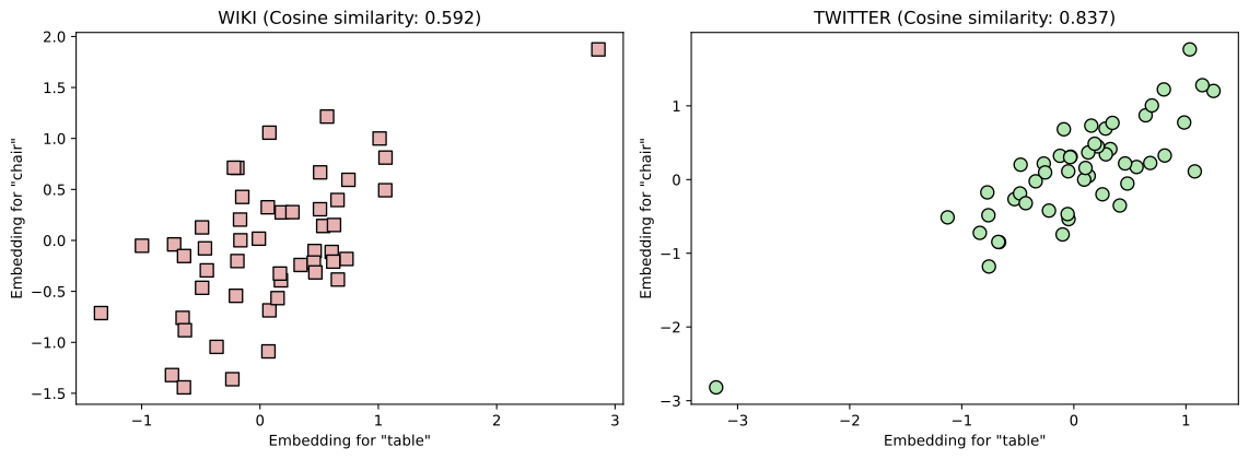

6. Model-Specific Neighbors

The contextual bias of a model becomes clear when we look at the words most similar to a technical term like "battery."

python

print('10 words most similar to "battery" in wiki:')
for w,cs in wiki.most_similar('battery'):
  print(f' {w:>15} with similarity {cs:.4f}')

print('\nAnd in twitter:')
for w,cs in twit.most_similar('battery'):
  print(f' {w:>15} with similarity {cs:.4f}')

Out · stdout

10 words most similar to "battery" in wiki:
       batteries with similarity 0.8322
    rechargeable with similarity 0.7258
     lithium-ion with similarity 0.7083
          weapon with similarity 0.6928

18 more lines

         machine with similarity 0.6788
       lead-acid with similarity 0.6765
          device with similarity 0.6706
   anti-aircraft with similarity 0.6586
             gun with similarity 0.6580
        electric with similarity 0.6577

And in twitter:
charger with similarity 0.8721
cell with similarity 0.8216
batteries with similarity 0.8167
laptop with similarity 0.8139
batt with similarity 0.8043
charging with similarity 0.7881
replacement with similarity 0.7854
adapter with similarity 0.7587
phone with similarity 0.7572
charge with similarity 0.7499

7. Sentence Rank and OOV Analysis

When processing a full sentence, we often encounter words that exist in one model but might be missing (OOV) in another. Let's compare the indices for a famous sentence.

python

text = 'The quick brown fox jumps over the lazy dog'

import re
words = re.split(r'\s+',text.lower())

# index sequence in the two embeddings
wiki_idx = [wiki.key_to_index[w] if w in wiki.key_to_index else np.inf for w in words ]
twit_idx = [twit.key_to_index[w] if w in twit.key_to_index else np.inf for w in words ]


print(' Word |  Wiki | Twitter')
print('-'*23)
for o,w,t in zip(words,wiki_idx,twit_idx):
  print(f'{o:>5} | {w:>5} | {t:>5}')

Out · stdout

 Word | Wiki | Twitter

the | 0 | 13
quick | 2582 | 2156
brown | 1042 | 1871

6 more lines

 fox | 2106 | 4000
jumps | 11070 | 18014
over | 74 | 254
the | 0 | 13
lazy | 16531 | 2222
dog | 2926 | 1317

8. Correlation of Semantic Spaces

Finally, we can calculate the similarity for all pairs of words in the sentence and see if the two models agree on their semantic relationships. We quantify the distance of each pair from the "unity" line (where the two models agree perfectly) using the orthogonal projection of one vector onto another:

$\Delta = \left\| \mathbf{v} - \frac{\mathbf{v}' \mathbf{u}}{\mathbf{u}' \mathbf{u}} \mathbf{u} \right\|$

Where:

$\mathbf{u} = \begin{bmatrix} 1 \\ 1 \end{bmatrix}$ is the unity vector.
$\mathbf{v} = \begin{bmatrix} S_c(\text{wiki}) \\ S_c(\text{twit}) \end{bmatrix}$ is the vector of similarities from both models.
$\Delta$ represents the perpendicular distance from the identity line, which we use to color-code our visualization (scaling by $5\Delta$ ).

python

# get all unique inter-word similarities

plt.figure(figsize=(9,7))

for i in range(0,len(words)):
  for j in range(i+1,len(words)):

    # skip identity
    if words[i]==words[j]: continue

    # skip if any word is missing in either model
    if np.isinf(wiki_idx[i]) or np.isinf(wiki_idx[j]) or \
       np.isinf(twit_idx[i]) or np.isinf(twit_idx[j]):
        continue

    # calculate the cosine similarities
    cs_wiki = wiki.similarity(words[i],words[j])
    cs_twit = twit.similarity(words[i],words[j])

    # calculate distance from unity (Delta)
    v = np.array([cs_wiki,cs_twit])
    u = np.array([1,1])
    delta = np.linalg.norm( v - (np.dot(v,u)/np.dot(u,u))*u )

    # plot
    plt.plot(cs_wiki,cs_twit,'ks',markerfacecolor=plt.cm.plasma(5*delta),markersize=12,alpha=.8)
    plt.text(cs_wiki,cs_twit+.01,f'{words[i]}-{words[j]}',horizontalalignment='center',fontsize=10)


# plot the unity line
xylims = [.05,.95]
plt.plot(xylims,xylims,'--',color=[.4,.4,.4],zorder=-30)

# final adjustments
plt.gca().set(xlim=xylims,ylim=xylims,xlabel='Wiki inter-word similarities',\
              ylabel='Twitter inter-word similarities',title='Inter-word similarities')
plt.show()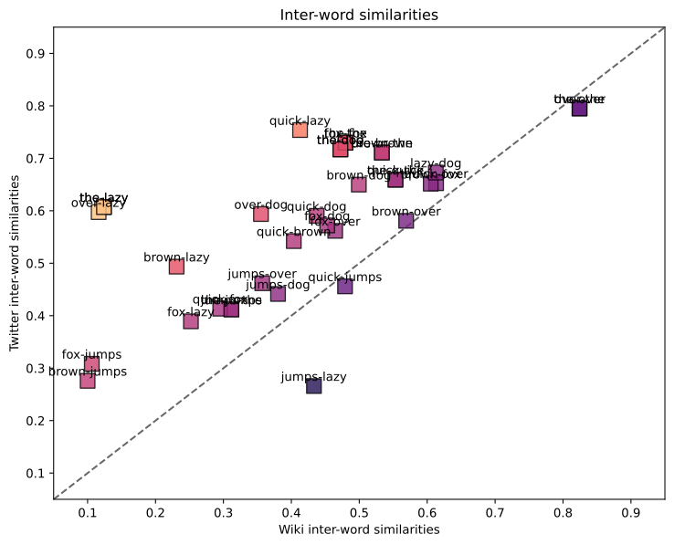

Key Take-home Points

Context Matters: Training on Wikipedia (formal) vs. Twitter (informal) leads to different semantic neighbors for the same word.
Vocabulary Gaps: Twitter's vocabulary is much larger but contains more slang and specialized tokens.
Semantic Consistency: Despite training on different data, the relative similarity between core concepts (like 'table' and 'chair') often remains correlated.
OOV Handling: Modern NLP must account for words that are missing from static embedding dictionaries.