Adapted from A deep understanding of AI language model mechanisms — https://udemy.com/course/dullms_x
1. Initializing the Model
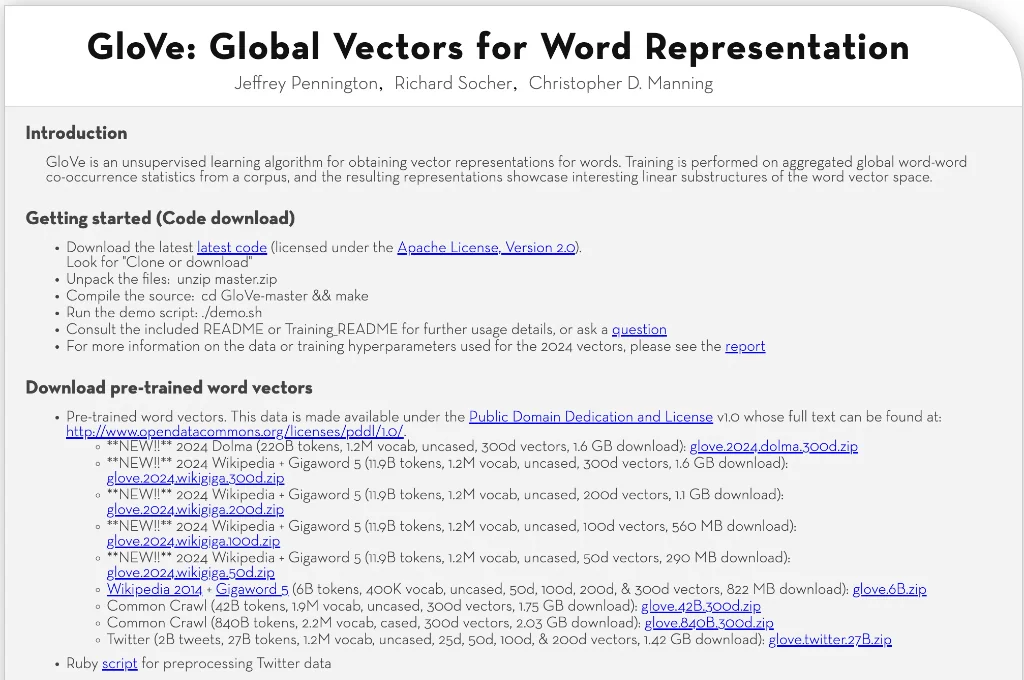
We'll begin by downloading a pretrained GloVe model. For this lesson, we use the 50-dimensional Wikipedia version, which provides a good balance between semantic depth and memory efficiency.
# download a small GloVe model (Wikipedia + Gigaword, 50D)

# NOTE: If you get errors importing, run the following !pip... line,
# then restart your session (from Runtime menu) and comment out the pip line.
# !pip install gensim

import gensim.downloader as api
glove = api.load('glove-wiki-gigaword-50')[==================================================] 100.0% 66.0/66.0MB downloadedEnvironment Setup
Next, we import our data science stack and configure the notebook to render high-quality SVG plots.
import numpy as np
import scipy
import matplotlib.pyplot as plt
from matplotlib.gridspec import GridSpec

# svg plots
import matplotlib_inline.backend_inline
matplotlib_inline.backend_inline.set_matplotlib_formats('svg')
2. Inspecting the GloVe Object
Let's examine the glove variable to see the methods and attributes it exposes for semantic analysis.
Explore the glove variable
# check the properties and methods
dir(glove)['__class__',
'__contains__',
'__delattr__',
'__dict__',
'__dir__',92 more lines
 '__doc__',
 '__eq__',
 '__format__',
 '__ge__',
 '__getattribute__',
 '__getitem__',
 '__getstate__',
 '__gt__',
 '__hash__',
 '__init__',
 '__init_subclass__',
 '__le__',
 '__len__',
 '__lt__',
 '__module__',
 '__ne__',
 '__new__',
 '__reduce__',
 '__reduce_ex__',
 '__repr__',
 '__setattr__',
 '__setitem__',
 '__sizeof__',
 '__str__',
 '__subclasshook__',
 '__weakref__',
 '_adapt_by_suffix',
 '_load_specials',
 '_log_evaluate_word_analogies',
 '_save_specials',
 '_smart_save',
 '_upconvert_old_d2vkv',
 '_upconvert_old_vocab',
 'add_lifecycle_event',
 'add_vector',
 'add_vectors',
 'allocate_vecattrs',
 'closer_than',
 'cosine_similarities',
 'distance',
 'distances',
 'doesnt_match',
 'evaluate_word_analogies',
 'evaluate_word_pairs',
 'expandos',
 'fill_norms',
 'get_index',
 'get_mean_vector',
 'get_normed_vectors',
 'get_vecattr',
 'get_vector',
 'has_index_for',
 'index2entity',
 'index2word',
 'index_to_key',
 'init_sims',
 'intersect_word2vec_format',
 'key_to_index',
 'lifecycle_events',
 'load',
 'load_word2vec_format',
 'log_accuracy',
 'log_evaluate_word_pairs',
 'mapfile_path',
 'most_similar',
 'most_similar_cosmul',
 'most_similar_to_given',
 'n_similarity',
 'next_index',
 'norms',
 'rank',
 'rank_by_centrality',
 'relative_cosine_similarity',
 'resize_vectors',
 'save',
 'save_word2vec_format',
 'set_vecattr',
 'similar_by_key',
 'similar_by_vector',
 'similar_by_word',
 'similarity',
 'similarity_unseen_docs',
 'sort_by_descending_frequency',
 'unit_normalize_all',
 'vector_size',
 'vectors',
 'vectors_for_all',
 'vectors_norm',
 'vocab',
 'wmdistance',
 'word_vec',
 'words_closer_than']
3. Vocabulary Overview
The model contains a massive dictionary of unique tokens. We can verify the total size and peek at the most frequent words (typically stop-words and punctuation).
print(f'The dictionary contains {len( glove.key_to_index.keys())} items.' )
list(glove.key_to_index.keys())[:50]The dictionary contains 400000 items.['the',
',',
'.',
'of',
'to',45 more lines
 'and',
 'in',
 'a',
 '"',
 "'s",
 'for',
 '-',
 'that',
 'on',
 'is',
 'was',
 'said',
 'with',
 'he',
 'as',
 'it',
 'by',
 'at',
 '(',
 ')',
 'from',
 'his',
 "''",
 '``',
 'an',
 'be',
 'has',
 'are',
 'have',
 'but',
 'were',
 'not',
 'this',
 'who',
 'they',
 'had',
 'i',
 'which',
 'will',
 'their',
 ':',
 'or',
 'its',
 'one',
 'after']
4. Vocabulary Sampling
To understand the variety of data in the model, let's pull 10 random indices and see which words they correspond to.
Explore the vocab
# print 10 words at random
for idx in np.random.randint(0,len(glove.key_to_index),10):
print(f'Index {idx:>6} is "{glove.index_to_key[idx]}"')Index 391518 is "8,470"
Index 213482 is "creacion"
Index 119937 is "mccoury"
Index 278063 is "leukerbad"
Index 40971 is "rahlves"5 more lines
Index 157519 is "vitelic"
Index  68169 is "yuletide"
Index 371087 is "congo-kinshasa"
Index  29437 is "acutely"
Index 276666 is "ferridge"
Word Length Statistics
We can also look at the statistical distribution of character counts across the entire 400,000-word dataset.
# distribution of token character lengths
token_lengths = np.zeros(len( glove.key_to_index.keys()),dtype=int)
for idx,word in enumerate( glove.key_to_index.keys() ):
  token_lengths[idx] = len(word)

# counts for the bar plot
uniqVals,uniqCounts = np.unique(token_lengths,return_counts=True)


# visualize the distribution of lengths
plt.figure(figsize=(12,4))
plt.bar(uniqVals,np.log(uniqCounts),width=uniqVals[1]-uniqVals[0],facecolor=[.9,.7,.9],edgecolor='k')
plt.gca().set(xlabel='Word length (num characters)',ylabel='Count')

plt.show()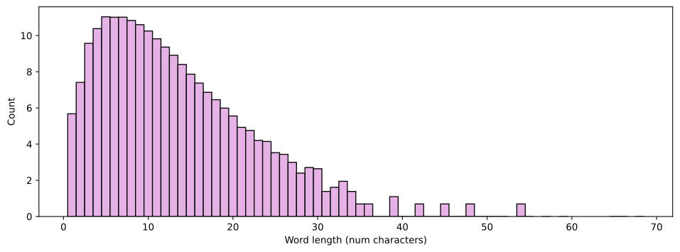
5. The Embeddings Matrix
The core of the model is the embeddings matrix, where every row represents a word and every column is a semantic dimension.
Explore the embeddings matrix
# size of the embeddings matrix
print(f'The embeddings matrix is {glove.vectors.shape}')

print(f'The word "apple" has index #{glove.key_to_index["apple"]}')

# can also access it this way:
glove.get_index('apple')The embeddings matrix is (400000, 50)
The word "apple" has index #32923292Weight Visualization
Visualizing the raw weights of the matrix provides a sense of the dense, continuous nature of the word representations.
plt.figure(figsize=(12,4))
plt.imshow(glove.vectors.T,vmin=-1,vmax=1,aspect='auto')
plt.gca().set(ylabel='Dimension',xlabel='Word index',title='Embeddings matrix')
plt.colorbar(pad=.01)
plt.show()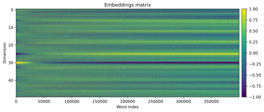
Global Distribution
We can also analyze the mean and variance of the values in the matrix to ensure the vectors are well-behaved.
# mean and std across each embedding dim
emb_mean = glove.vectors.mean(axis=1)
emb_std  = glove.vectors.std(axis=1)


# seaborn has nice visualization routines
import seaborn as sns
import pandas as pd # though seaborn only works on pandas dataframes :/

df = pd.DataFrame(np.vstack((emb_mean,emb_std)).T,columns=['Mean','std'])

sns.jointplot(x='Mean',y='std',data=df,alpha=.2)
plt.show()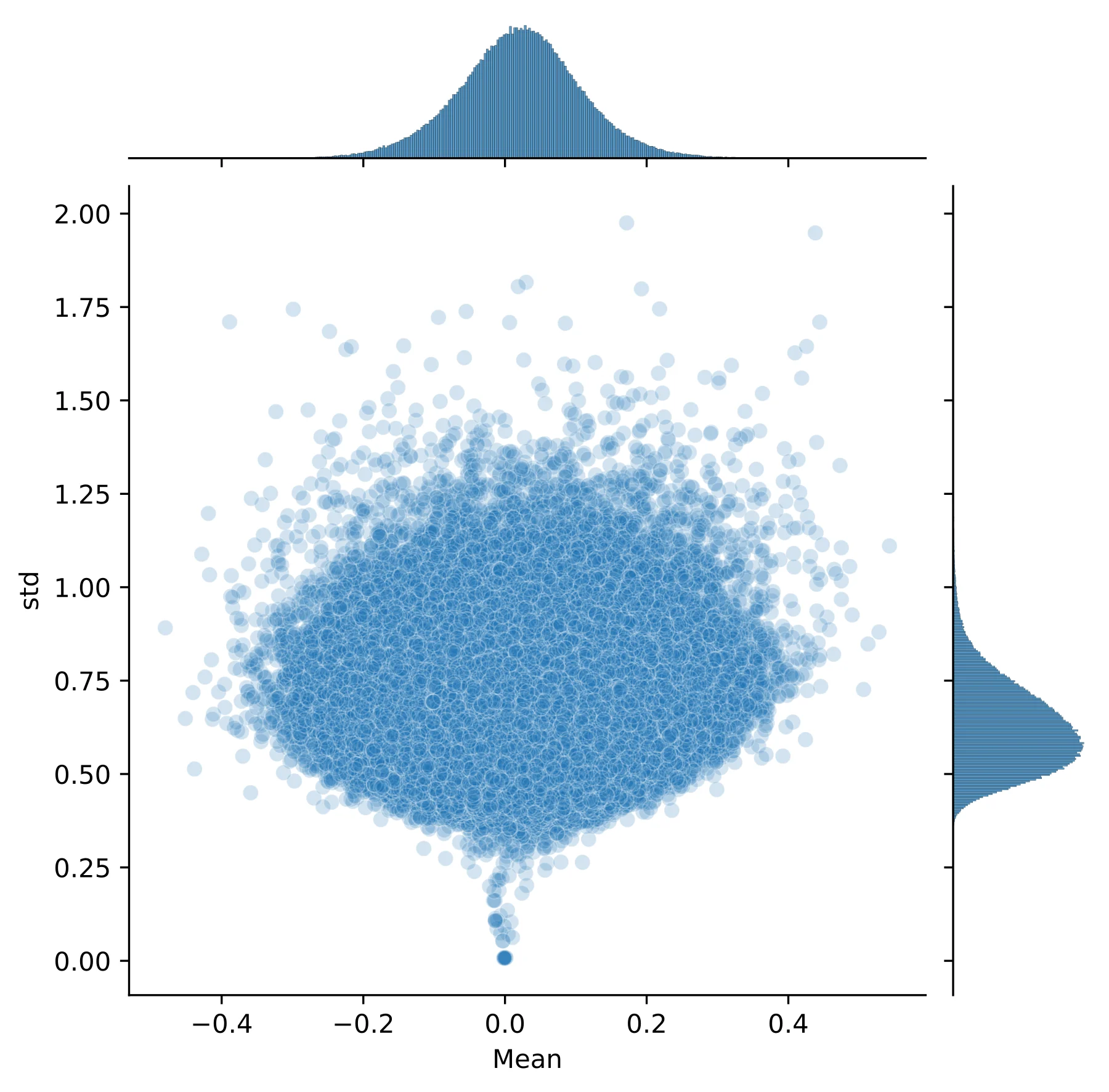
6. Individual Vector Extraction
Let's zoom in on a specific word to see its actual 50-dimensional coordinate in the vector space.
Explore individual embeddings vectors
# pick a word
word = 'banana'

# get its index in the embeddings matrix
wordidx = glove.key_to_index[word]

# get the embedding vector
thisWordVector = glove.vectors[wordidx,:]

# inspect the vector
print(f'The embedding vector for "{word}" is\n {thisWordVector}')The embedding vector for "banana" is
[-0.25522 -0.75249 -0.86655 1.1197 0.12887 1.0121 -0.57249
-0.36224 0.44341 -0.12211 0.073524 0.21387 0.96744 -0.068611
0.51452 -0.053425 -0.21966 0.23012 1.043 -0.77016 -0.16753
-1.0952 0.24837 0.20019 -0.40866 -0.48037 0.10674 0.53164 more lines
  1.111    -0.19322   1.4768   -0.51783  -0.79569   1.7971   -0.33392
 -0.14545  -1.5454    0.0135    0.10684  -0.30722  -0.54572   0.38938
  0.24659  -0.85166   0.54966   0.82679  -0.68081  -0.77864  -0.028242
-0.82872 ]# even easier ;)
thisWordVector = glove[word]
print(f'The embedding vector for "{word}" is\n {thisWordVector}')The embedding vector for "banana" is
[-0.25522 -0.75249 -0.86655 1.1197 0.12887 1.0121 -0.57249
-0.36224 0.44341 -0.12211 0.073524 0.21387 0.96744 -0.068611
0.51452 -0.053425 -0.21966 0.23012 1.043 -0.77016 -0.16753
-1.0952 0.24837 0.20019 -0.40866 -0.48037 0.10674 0.53164 more lines
  1.111    -0.19322   1.4768   -0.51783  -0.79569   1.7971   -0.33392
 -0.14545  -1.5454    0.0135    0.10684  -0.30722  -0.54572   0.38938
  0.24659  -0.85166   0.54966   0.82679  -0.68081  -0.77864  -0.028242
 -0.82872 ]
Vector Fingerprint
Plotting the dimensions of a single vector highlights the unique "fingerprint" the model uses to differentiate it from other words.
# visualize it
plt.figure(figsize=(10,4))
plt.plot(glove.vectors[wordidx,:],'ks',markersize=10,markerfacecolor=[.7,.7,.9])

plt.xlabel('Dimension')
plt.title(f'Embedding vector for "{word}"')
plt.show()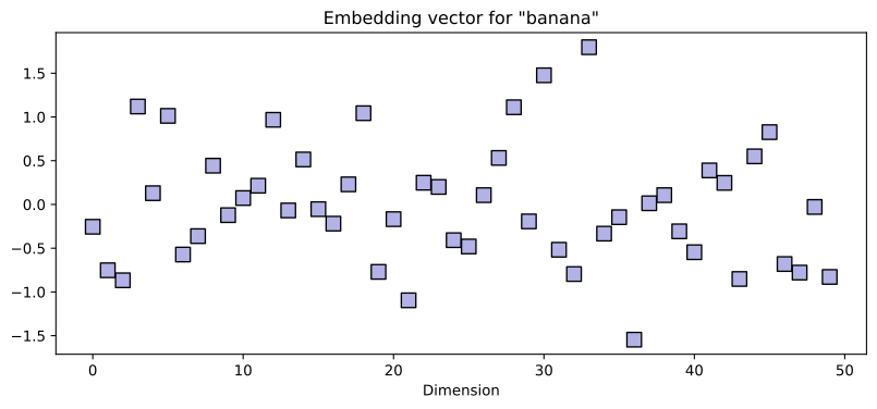
7. Semantic Comparison
The power of embeddings comes from comparison. By plotting multiple words on the same axes, we can see how they align or diverge. To quantify this relationship, we use Cosine Similarity, which measures the cosine of the angle between two vectors:
Where:
- is the dot product of the vectors.
- and are the magnitudes (Euclidean norms).
- The result ranges from -1 (opposite) to 1 (identical), with 0 indicating orthogonality (no relationship).
Relationships across embedding vectors
# pick three words
word1 = 'banana'
word2 = 'apple'
word3 = 'cosmic'


# setup the figure subplot geometry
fig = plt.figure(figsize=(10,7))
gs = GridSpec(2,2)
ax0 = fig.add_subplot(gs[0,:])
ax1 = fig.add_subplot(gs[1,0])
ax2 = fig.add_subplot(gs[1,1])

# plot the embeddings by dimension
for idx,word in enumerate([word1,word2,word3]):
  ax0.plot(glove[word],'s-',label=word)

ax0.set(xlabel='Dimension',title='Embeddings',xlim=[-1,glove.vectors.shape[1]+1])
ax0.legend()


# plot the embeddings by each other
cossim = glove.similarity(word1,word2)
ax1.plot(glove[word1],glove[word2],'ko',markerfacecolor=[.9,.7,.7])
ax1.set(xlabel=word1,ylabel=word2,title=f'Cosine similarity = {cossim:.3f}')

cossim = glove.similarity(word1,word3)
ax2.plot(glove[word1],glove[word3],'ko',markerfacecolor=[.7,.9,.7])
ax2.set(xlabel=word1,ylabel=word3,title=f'Cosine similarity = {cossim:.3f}')

# final touches
plt.tight_layout()
plt.show()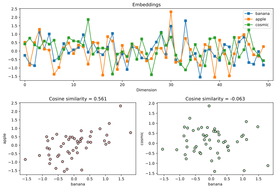
8. Similarity Operations
Finally, we can use built-in methods to discover semantically related words or find the "odd one out" in a list of tokens.
Methods to identify similar and dissimilar words
# most similar words ("similar" is high cosine similarity)
glove.most_similar('fashion',topn=9)[('style', 0.760734498500824),
('fashions', 0.7528777122497559),
('designer', 0.7515820860862732),
('chic', 0.7511471509933472),
('designers', 0.7450659275054932),4 more lines
 ('shows', 0.7221302390098572),
 ('couture', 0.7165465354919434),
 ('glamour', 0.7155618667602539),
('show', 0.7142423391342163)]# One these things is not like the others...
lists = [ [ 'apple','banana','pirate','peach' ],
[ 'apple','banana','peach','kiwi','starfruit' ],
[ 'apple','banana','pirate','peach','kiwi','starfruit' ],
[ 'apple','banana','orange','kiwi' ]
]
for l in lists:
print(f'In the word list {l}:')
print(f' The most similar word is "{glove.most_similar(l,topn=1)[0][0]}"')
print(f' and the non-matching word is "{glove.doesnt_match(l)}"\n')In the word list ['apple', 'banana', 'pirate', 'peach']:
The most similar word is "mango"
and the non-matching word is "pirate"
In the word list ['apple', 'banana', 'peach', 'kiwi', 'starfruit']:10 more lines
 The most similar word is "mango"
and the non-matching word is "starfruit"

In the word list ['apple', 'banana', 'pirate', 'peach', 'kiwi', 'starfruit']:
The most similar word is "mango"
and the non-matching word is "starfruit"

In the word list ['apple', 'banana', 'orange', 'kiwi']:
The most similar word is "juice"
and the non-matching word is "kiwi"
Key Take-home Points
- Study of Texts: GloVe embeddings are powerful tools for studying semantic relations and statistical patterns across large corpora.
- Static Nature: Once trained, embedding vectors are fixed (static), meaning the word "bank" has the same vector regardless of context.
- Legacy for LLMs: GloVe is rarely used in modern LLMs because of its word-based vocabulary and inability to handle out-of-vocabulary (OOV) tokens effectively.
- Broad Applications: Cosine similarity remains a fundamental metric in language modeling, search engines, and computational linguistics.