8. Position Embeddings

Adapted from A deep understanding of AI language model mechanisms — https://udemy.com/course/dullms_x

Why Do Models Need Position Embeddings?

Large Language Models (Transformers) have no built-in method of representing time, token positions in a text, or relative positions (ordinal distances) among tokens. Without a mechanism to track positions, a Transformer treats any input as a simple "bag of words"—meaning sentences like "the dog bit the man" and "the man bit the dog" would produce identical representation vectors.

To see why sequence order and relative distance are so critical, consider the following sentence:

The Coreference Challenge: "Hazelnuts are used as a snack food, in baking and desserts, and in breakfast cereals such as muesli. In confectionery, they..."

For a model to find out what "they" refers to (resolving coreference back to Hazelnuts), the self-attention mechanism must be able to weight different tokens according to their exact positions in the text. Without positional context, "they" would attend equally to muesli, desserts, cereals, or Hazelnuts, with no spatial awareness of where they sit in the sequence.

Position vectors solve this by allowing models to weight different tokens according to their positions in a text, enabling the self-attention mechanism to capture structure, grammar, and long-range dependencies.

What is "Time" in an LLM and How Do We Find It?

When we discuss "time" in the context of Large Language Models, we are not talking about wall-clock time. Instead, "time" refers to the ordinal sequence index of a token in a text (i.e., Token 0, Token 1, Token 2, etc.).

Because transformers process all input tokens in parallel rather than step-by-step (unlike older recurrent architectures like RNNs or LSTMs), they have no natural sense of sequence progression. To them, a sentence is initially just an unordered set of words.

How Do We "Find Out" Time?

To give the model a sense of time, we inject a coordinate system directly into the inputs:

1. Assigning Timestamps: For every token index $t$ in the input sequence, we generate or look up a unique positional encoding vector ($PE_t$) that represents that specific coordinate.
2. Vector Addition: We add this position vector directly to the semantic word embedding vector ($WE_t$): $$E_t = WE_t + PE_t$$
3. Downstream Decoding: When the combined vector $E_t$ goes through the transformer's self-attention layers, the projection matrices (Query, Key, Value) can mathematically isolate and decode these positional coordinates. This allows the model to compute exactly how far apart any two tokens are, reconstructing the flow of "time" across the text.

Where Do Position Embeddings Come From?

To inject positional awareness, we add position embeddings directly to our standard word embeddings. These vectors generally come from one of two approaches:

1. Trained (Learned) Positional Embeddings

• How it Works: Position vectors are initialized as random numbers and optimized through gradient descent alongside other model parameters during training.
• Key Benefits: Fits the specific training data distribution perfectly, capturing custom geometric relationships.
• Trade-offs & Challenges: Adds weights to the model that must be trained, and cannot extrapolate beyond the fixed context window length defined during training (e.g., 1024 tokens in GPT-2).

2. Predefined (Fixed) Positional Embeddings

• How it Works: Position vectors are generated statically using mathematical trigonometric formulas (specifically sine and cosine waves of varying frequencies).
• Key Benefits: Zero extra parameters to train (saving computational overhead), and has the potential to extrapolate to longer sequences.
• Trade-offs & Challenges: Natural language is highly complex and might require complicated combinations of embeddings (similar to a Fourier transform of a square wave) that predefined trig formulas cannot adapt to as perfectly as learned parameters.

1. Setup and Environment

We'll start by importing our standard data science tools and configuring the plotting backend for high-quality SVG outputs.

import numpy as np
import matplotlib.pyplot as plt

# higres plots
import matplotlib_inline.backend_inline
matplotlib_inline.backend_inline.set_matplotlib_formats('svg')

2. Loading GPT-2

We'll load the pretrained GPT-2 model to inspect its internal embedding layers, specifically focusing on the wpe (word position embedding) layer.

# load the model
from transformers import GPT2Model
gpt2 = GPT2Model.from_pretrained('gpt2')
gpt2

/Users/drippy/.pyenv/versions/3.12.6/lib/python3.12/site-packages/tqdm/auto.py:21: TqdmWarning: IProgress not found. Please update jupyter and ipywidgets. See https://ipywidgets.readthedocs.io/en/stable/user_install.html
  from .autonotebook import tqdm as notebook_tqdm

GPT2Model(
  (wte): Embedding(50257, 768)
  (wpe): Embedding(1024, 768)
  (drop): Dropout(p=0.1, inplace=False)
  (h): ModuleList(

    (0-11): 12 x GPT2Block(
      (ln_1): LayerNorm((768,), eps=1e-05, elementwise_affine=True)
      (attn): GPT2Attention(
        (c_attn): Conv1D(nf=2304, nx=768)
        (c_proj): Conv1D(nf=768, nx=768)
        (attn_dropout): Dropout(p=0.1, inplace=False)
        (resid_dropout): Dropout(p=0.1, inplace=False)
      )
      (ln_2): LayerNorm((768,), eps=1e-05, elementwise_affine=True)
      (mlp): GPT2MLP(
        (c_fc): Conv1D(nf=3072, nx=768)
        (c_proj): Conv1D(nf=768, nx=3072)
        (act): NewGELUActivation()
        (dropout): Dropout(p=0.1, inplace=False)
      )
    )
  )
  (ln_f): LayerNorm((768,), eps=1e-05, elementwise_affine=True)
)

3. Position Embedding Matrix (WPE)

To understand how a transformer models position, we must zoom in on its dual embedding setup:

1. Word Token Embeddings (WTE)*: Maps the semantic identity* of a token (e.g., the word "dog" to its conceptual meaning). GPT-2's vocabulary consists of 50,257 tokens, so its WTE matrix is sized (50257, 768).
2. Word Position Embeddings (WPE)*: Maps the spatial coordinate* of a token (e.g., its index $t$ in the text stream). GPT-2 has a maximum context window of 1,024, so its WPE matrix is sized (1024, 768).

How Do We "Find" the Position Vectors?

Retrieving the position vector for any word in a sequence is incredibly efficient. It is implemented as a simple row lookup (or $O(1)$ matrix indexing) based on the token's position index:

• Index Generation: When you feed a sequence of length $N$ into the model, the framework automatically generates a sequential integer coordinate array: [0, 1, 2, ..., N-1].
• Matrix Slicing: For a token sitting at position $t$, the model extracts the $t$-th row of the WPE weight matrix.
• In PyTorch: This is handled under the hood by a simple nn.Embedding(1024, 768) layer. Under the hood, this layer is simply a standard 2D weight matrix. Calling it with an index array t retrieves the corresponding slices:

  # PyTorch equivalent lookup:
  position_vectors = gpt2.wpe(torch.arange(sequence_length))

Let's extract the active weight matrix to examine the weights directly:

# position embeddings
positions = gpt2.wpe.weight.detach().numpy()

Matrix Visualization

Visualizing the full position embedding matrix allows us to see if there are any global patterns or structural shifts as we move from the beginning to the end of the context window.

# check the size of this matrix
positions.shape

(1024, 768)

# visualize the matrix
plt.figure(figsize=(10,4))
plt.imshow(positions.T,aspect='auto',vmin=-.2,vmax=.2)
plt.gca().set(xlabel='Token position',ylabel='Dimensions',title='GPT-2 position embedding matrix')
plt.show()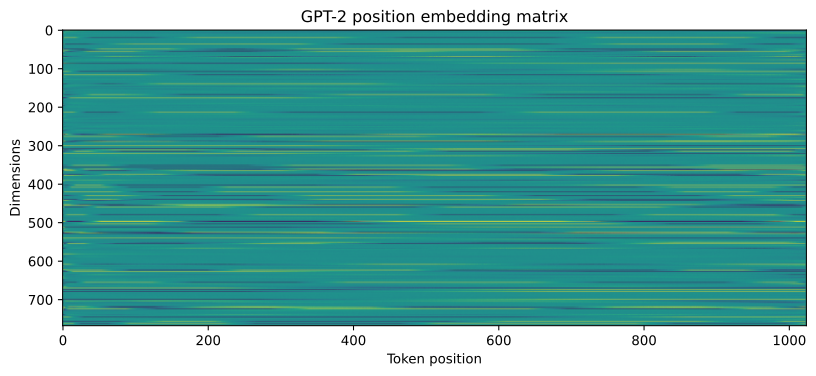

4. Visualizing Position Vectors

Let's examine individual columns of the position embedding matrix. Each vector represents the unique "signature" for a specific position in the 1024-token context.

_,axs = plt.subplots(3,4,figsize=(16,6))

# pick random vectors
for a in axs.flatten():

  # a random position embedding vector
  randidx = np.random.randint(positions.shape[1])

  # and plot it
  a.plot(positions[:,randidx],'k',label=f'Position index {randidx}')
  a.axhline(0,linestyle='--',color='gray',zorder=-3)

  a.set(xticks=[],yticks=[0],xlim=[0,positions.shape[0]])
  a.legend(fontsize=10)


# x-axis label on one plot
a.set_xlabel('Start of text <---> end of context window',fontsize=12)
plt.tight_layout()
plt.show()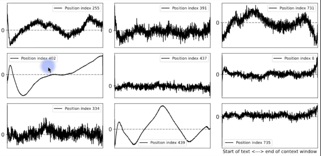

Interpreting the Position Vector Plots

Looking closely at these "wiggly lines" (the active position embeddings mapped across the context window), we can extract some highly intuitive observations about how a transformer encodes sequence coordinates:

• Understanding the Coordinates:
• X-Axis (Sequence Index): Represents the ordinal token positions in the input text. 0 on the left corresponds to the very start of the text. As we move right, we traverse the model's context window (the maximum sequence length, e.g., 1024 tokens in GPT-2, or up to 100,000 tokens in GPT-4 variants).
• Y-Axis (Weighting Value): Represents the weight or bias added to the token embedding at each position.
• Analyzing Specific Position Vectors:
• Vector 402 (Recency Gradient): This vector exhibits a strong positive weight toward the right side (recent tokens) and negative weights going further left (older tokens). This functions as a linear importance decay over the sequence, helping the model naturally track relative distance or time. Interestingly, it also features a sharp peak at index 0—this enables the model to tie terminal states (like a summary at the end) back to the initial context established at the very beginning of the sequence.
• Mid-Sequence Focus: Other vectors (like those with a central peak) display maximum weighting in the middle of the context window and neutral values at the ends. This allows the model to prioritize or highlight tokens appearing strictly in the middle of a passage.

A Note on "Attention": While we are tempted to say these vectors help the model attend to various ordinal positions, the word "attention" is reserved for the active Query-Key-Value matching mechanism in transformers. However, position embeddings serve as the vital coordinate system that makes that attention mechanism sequence-aware.

• Decoding the Signs and Values:
• Neutral (0): An embedding value of zero is clean and interpretable: it means this specific dimension provides absolutely no position-based bias for that token index.
• Positive vs. Negative: The signs do not trivially correlate to "increasing" or "decreasing" token activation or select probabilities. Instead, the downstream impact depends entirely on how these signs align with the weights of the query, key, and value projection matrices as the model processes the combined embeddings.

5. Analyzing Learned Similarities

Are nearby positions more similar to each other than distant ones? We'll calculate the cosine similarity between position vectors to visualize the model's "temporal" awareness.

# cosine similarities for "time series" (token index)
Pnorm1 = positions / np.linalg.norm(positions,axis=1,keepdims=True)
cossim_tokens = Pnorm1 @ Pnorm1.T

# cosine similarities across embedding dimensions
Pnorm0 = positions / np.linalg.norm(positions,axis=0,keepdims=True)
cossim_embeds = Pnorm0.T @ Pnorm0


# draw the images
fig,axs = plt.subplots(1,2,figsize=(12,5))

h = axs[0].imshow(cossim_tokens,vmin=-1,vmax=1)
axs[0].set(xlabel='Token index ("time")',ylabel='Token index ("time")',title='$S_c$ over "time"')
ch = fig.colorbar(h,ax=axs[0],pad=.02,fraction=.046)
ch.ax.tick_params(labelsize=10)
ch.ax.set_yticks(np.arange(-1,1.1,.5))

h = axs[1].imshow(cossim_embeds,vmin=-1,vmax=1)
axs[1].set(xlabel='Embedding index',ylabel='Embedding index',title='$S_c$ across embeddings')
ch = fig.colorbar(h,ax=axs[1],pad=.02,fraction=.046)
ch.ax.tick_params(labelsize=10)
ch.ax.set_yticks(np.arange(-1,1.1,.5))

plt.tight_layout()
plt.show()

Deconstructing the Mathematical Operations

This concise block of NumPy operations implements a highly optimized method for calculating millions of cosine similarities simultaneously using vector operations. Let's break down the mechanics line-by-line:

1. Defining Cosine Similarity in Vector Terms

For two arbitrary vectors $\mathbf{u}$ and $\mathbf{v}$, the cosine similarity is defined as: $$S_c(\mathbf{u}, \mathbf{v}) = \frac{\mathbf{u} \cdot \mathbf{v}}{\|\mathbf{u}\| \|\mathbf{v}\|} = \left(\frac{\mathbf{u}}{\|\mathbf{u}\|}\right) \cdot \left(\frac{\mathbf{v}}{\|\mathbf{v}\|}\right)$$ This formula tells us that cosine similarity is equivalent to the dot product of two L2-normalized (unit length) vectors. This is the key mathematical trick used to write such efficient, clean code!

2. Cosine Similarity Over "Time" (Token Positions)

Our goal here is to find the similarity between individual token positions (e.g., comparing the coordinate vector at position $5$ with the coordinate vector at position $50$). This matches the rows of our matrix.

• Line 1: L2-Normalization of Rows

  Pnorm1 = positions / np.linalg.norm(positions, axis=1, keepdims=True)

• np.linalg.norm(..., axis=1): Calculates the magnitude (L2-norm) of each row vector (across the 768 columns).
• keepdims=True: Transforms the output from a flat array of shape (1024,) to a 2D column vector of shape (1024, 1). This is crucial for NumPy broadcasting to cleanly divide each element in positions by its row's specific norm.
• Pnorm1: The resulting matrix contains the same position weights, but every row is now a unit vector (length of $1.0$).
• Line 2: Row-wise Dot Products via Matrix Multiplication

  cossim_tokens = Pnorm1 @ Pnorm1.T

• @: Performs matrix multiplication (dot products). We multiply Pnorm1 of shape (1024, 768) by its transpose Pnorm1.T of shape (768, 1024).
• The resulting dot product in each cell $(i, j)$ yields a (1024, 1024) matrix, containing the exact cosine similarity between Token position $i$ and Token position $j$.

Concrete Numerical Example (Toy 3×2 Matrix)

To see exactly how these two lines work in memory, let's step through them using a toy matrix of 3 token positions with 2 embedding dimensions:

• Step 1: Calculating the Row Norms (np.linalg.norm(..., axis=1)) We compute the L2 magnitude ($\sqrt{x^2 + y^2}$) for each of the three rows:
• Row 0: $\sqrt{3^2 + 4^2} = 5.0$
• Row 1: $\sqrt{0^2 + 5^2} = 5.0$
• Row 2: $\sqrt{1^2 + 1^2} = \sqrt{2} \approx 1.414$

Setting keepdims=True outputs a 2D column vector of shape (3, 1): $$\text{Norms} = \begin{bmatrix} 5.0 \\ 5.0 \\ 1.414 \end{bmatrix}$$

• Step 2: Division Broadcasting (Line 1 Output) NumPy divides each row in our input matrix by its corresponding row norm to yield Pnorm1*: $$Pnorm1 = \begin{bmatrix} 3 / 5.0 & 4 / 5.0 \\ 0 / 5.0 & 5 / 5.0 \\ 1 / 1.414 & 1 / 1.414 \end{bmatrix} = \begin{bmatrix} 0.6 & 0.8 \\ 0.0 & 1.0 \\ 0.707 & 0.707 \end{bmatrix}$$ Note: Every row in Pnorm1 is now a unit vector (norm of 1.0).*
• Step 3: Calculating Pnorm1.T (Transpose) We flip the axes of our normalized matrix to get a (2, 3) matrix: $$Pnorm1^T = \begin{bmatrix} 0.6 & 0.0 & 0.707 \\ 0.8 & 1.0 & 0.707 \end{bmatrix}$$
• Step 4: Dot Products via Matrix Product (Line 2 Output) We perform the matrix multiplication Pnorm1 @ Pnorm1.T: $$\begin{bmatrix} 0.6 & 0.8 \\ 0.0 & 1.0 \\ 0.707 & 0.707 \end{bmatrix} \times \begin{bmatrix} 0.6 & 0.0 & 0.707 \\ 0.8 & 1.0 & 0.707 \end{bmatrix} = \begin{bmatrix} 1.0 & 0.8 & 0.990 \\ 0.8 & 1.0 & 0.707 \\ 0.990 & 0.707 & 1.0 \end{bmatrix}$$
• Self-similarities (diagonal elements like (0,0), (1,1), (2,2)) are trivially 1.0.
• Pair similarities (off-diagonal elements like (0,1) similarity of 0.8) represent the exact cosine similarity between those token positions!

3. Cosine Similarity Across Embedding Dimensions

Our goal here is to analyze how similar the feature channels (columns) are to one another across all 1,024 steps of "time".

• Line 3: L2-Normalization of Columns

  Pnorm0 = positions / np.linalg.norm(positions, axis=0, keepdims=True)

• np.linalg.norm(..., axis=0): Computes the magnitude of each column vector (across the 1,024 rows).
• keepdims=True: Keeps the output shape as (1, 768) for correct column-wise division broadcasting.
• Line 4: Column-wise Dot Products

  cossim_embeds = Pnorm0.T @ Pnorm0

• We multiply the transposed normalized columns (768, 1024) by the original matrix (1024, 768).
• The result is a (768, 768) matrix showing the similarity of each embedding dimension to every other embedding dimension.

Interpreting the Learned Similarities

Let's break down the two heatmaps generated above:

• Cosine Similarity Across Embedding Dimensions (Right): This plot reveals how correlated different dimensions of the positional matrix are with one another. If certain columns show high similarity, those dimensions carry highly redundant positional signals.
• Cosine Similarity Over Token Index "Time" (Left): This is by far the more colorful and fascinating plot. If you think of the $1,000$ token positions as a progression of time (since we read text sequentially over time), this heatmap reveals the model's geometric temporal structure:
• The Dominant Diagonal Band: Neighboring token positions are highly correlated. A token at position $t$ is strongly aligned with its immediate neighbor at $t+1$, creating a smooth transition gradient.
• Rhythmic Alternating Bands: As you move off the diagonal, you see a clean, repeating pattern of yellow (correlated) and blue (anti-correlated) bands. Because the learned position curves tend to rise and fall periodically over the context window, their mutual similarities produce these beautiful wave-like rhythmic patterns.

6. Sinusoidal Positional Encoding

While GPT-2 learns its position embeddings, the original "Attention is All You Need" paper proposed a fixed formula using sine and cosine waves of varying frequencies.

positionsFormula = np.zeros_like(gpt2.wpe.weight.data)
d = positionsFormula.shape[1]

# token position ("time")
th = np.arange(positionsFormula.shape[0])

# create the vectors
for i in range(0,positionsFormula.shape[1],2):

  # denominator scaling factor
  denom = 10000 * (2i//2 / d)

  # define the embeddings
  positionsFormula[:,i]   = np.sin(th / denom)
  positionsFormula[:,i+1] = np.cos(th / denom)



### Formula Visualization
Plotting the sinusoidal embeddings reveals the elegant geometric structure that allows the model to attend to relative positions across long distances.

_,axs = plt.subplots(1,2,figsize=(12,4)) axs[0].imshow(positionsFormula.T,vmin=-1,vmax=1) axs[0].set(ylabel='Embedding dimensions',xlabel='Token order ("time")',title='All position embeddings')

pos2show = np.linspace(200,600,4,dtype=int) h = axs[1].plot(positionsFormula[:,pos2show]) axs[1].set(ylabel='Weight value',xlabel='Token order ("time")',xlim=[0,len(th)],title='A few position embeddings')

for i,p in enumerate(pos2show): axs[0].axhline(p,linestyle='--',color=h[i].get_color(),linewidth=1.8)

plt.tight_layout() plt.show()

### Visualizing the Sinusoidal Coordinate Grid

This plot illustrates the elegant geometric structure of the predefined sinusoidal positional encoding from the original transformer paper:

* All Position Embeddings (Left):
  * Here, the x-axis represents the token order (which we can think of as time).
  * The y-axis is the sorted embedding dimension, ordered by the frequency of the sine and cosine waves used to generate the vectors. You can clearly see high-frequency waves at the top transitioning to smooth, low-frequency curves at the bottom.
  * The horizontal dashed lines highlight the specific position dimensions selected for the plot on the right.

* A Few Position Embeddings (Right):
  * This plot shows the actual sine and cosine curves of the selected dimensions over the sequence length. This pre-defined wave matrix allows the model to calculate relative positions mathematically without needing to spend capacity learning them during training.

---

## 7. Comparing Learned vs. Fixed Embeddings

Finally, we'll plot the sinusoidal vectors in the same style as our learned GPT-2 vectors to compare their visual complexity and range.

sample plot as earlier with the learned embeddings

_,axs = plt.subplots(3,4,figsize=(16,6))

pick random vectors

for a in axs.flatten():

a random position embedding vector

randidx = np.random.randint(positions.shape[1])

and plot it

a.plot(positionsFormula[:,randidx],'k',label=f'Position index {randidx}') a.axhline(0,linestyle='--',color='gray',zorder=-3)

a.set(xticks=[],yticks=[0],xlim=[0,positions.shape[0]]) a.legend(fontsize=10)

x-axis label on one plot

a.set(xlabel='<-- present ... past -->') plt.tight_layout() plt.show()

---

### 💡 Key Take-home Points
*   Positional Context: Without position embeddings, a transformer would be a "bag of words" model, unable to tell the difference between "the dog bit the man" and "the man bit the dog."
*   Context Window: GPT-2's fixed position matrix limits its maximum sequence length to 1024 tokens.
*   Learned vs. Fixed: While fixed sinusoidal encodings allow for theoretically infinite sequences, learned embeddings (like GPT-2's) can adapt more specifically to the training data.
*   Locality Bias: In learned models, nearby positions typically show higher similarity, which helps the model maintain local coherence.