Matrix Plots
NOTE: Make sure to watch the video lecture, not all datasets are well suited for a heatmap or clustermap.
Imports
The Data
World Population Prospects publishes United Nations population estimates for all world countries and every year from 1950 to 2020, as well as projections for different scenarios (low, middle and high variants) from 2020 to 2100. The figures presented here correspond to middle variant projections for the given year.
https://www.ined.fr/en/everything_about_population/data/all-countries/?lst_continent=900&lst_pays=926
Source : Estimates for the current year based on data from the World Population Prospects. United Nations.
# 2020 Projections
df = pd.read_csv('country_table.csv')dfCountries
Birth rate
Mortality rate
Life expectancy
Infant mortality rate50 more lines
Growth rate
0
AFRICA
32.577
7.837
63.472
44.215
24.40
1
ASIA
15.796
7.030
73.787
23.185
8.44
2
EUROPE
10.118
11.163
78.740
3.750
0.38
3
LATIN AMERICA AND THE CARIBBEAN
15.886
6.444
75.649
14.570
8.89
4
NORTHERN AMERICA
11.780
8.833
79.269
5.563
6.11
5
OCEANIA
16.235
6.788
78.880
16.939
12.79
6
WORLD
17.963
7.601
72.766
27.492
10.36
Heatmap
df = df.set_index('Countries')dfBirth rate
Mortality rate
Life expectancy
Infant mortality rate
Growth rate43 more lines
Countries
AFRICA
32.577
7.837
63.472
44.215
24.40
ASIA
15.796
7.030
73.787
23.185
8.44
EUROPE
10.118
11.163
78.740
3.750
0.38
LATIN AMERICA AND THE CARIBBEAN
15.886
6.444
75.649
14.570
8.89
NORTHERN AMERICA
11.780
8.833
79.269
5.563
6.11
OCEANIA
16.235
6.788
78.880
16.939
12.79
WORLD
17.963
7.601
72.766
27.492
10.36# Clearly shows life expectancy in different units
sns.heatmap(df)<AxesSubplot:ylabel='Countries'>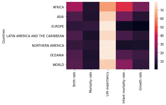
rates = df.drop('Life expectancy',axis=1)sns.heatmap(rates)<AxesSubplot:ylabel='Countries'>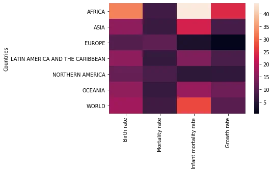
sns.heatmap(rates,linewidth=0.5)<AxesSubplot:ylabel='Countries'>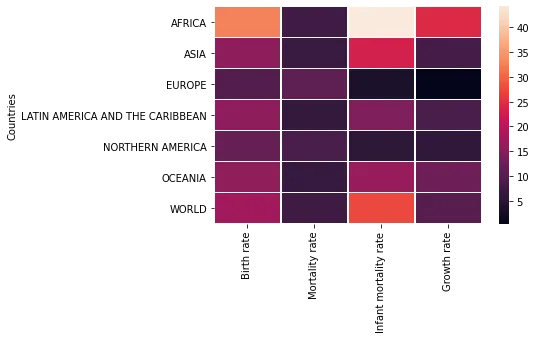
sns.heatmap(rates,linewidth=0.5,annot=True)<AxesSubplot:ylabel='Countries'>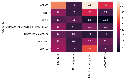
# Note how its not palette here
sns.heatmap(rates,linewidth=0.5,annot=True,cmap='viridis')<AxesSubplot:ylabel='Countries'>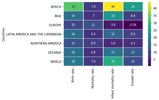
# Set colorbar based on value from dataset
sns.heatmap(rates,linewidth=0.5,annot=True,cmap='viridis',center=40)<AxesSubplot:ylabel='Countries'>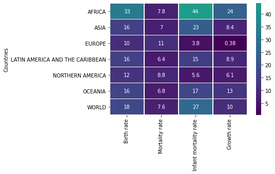
# Set colorbar based on value from dataset
sns.heatmap(rates,linewidth=0.5,annot=True,cmap='viridis',center=1)<AxesSubplot:ylabel='Countries'>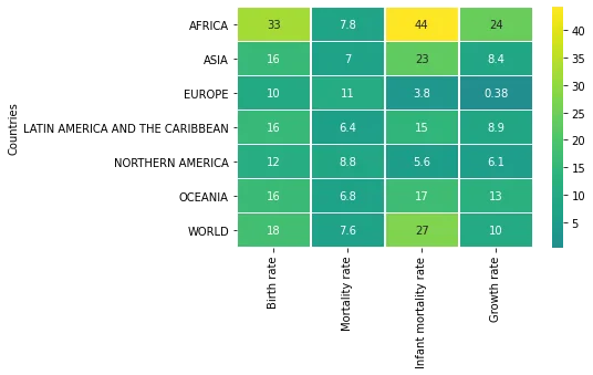
Clustermap
Plot a matrix dataset as a hierarchically-clustered heatmap.
sns.clustermap(rates)<seaborn.matrix.ClusterGrid at 0x158e27976c8>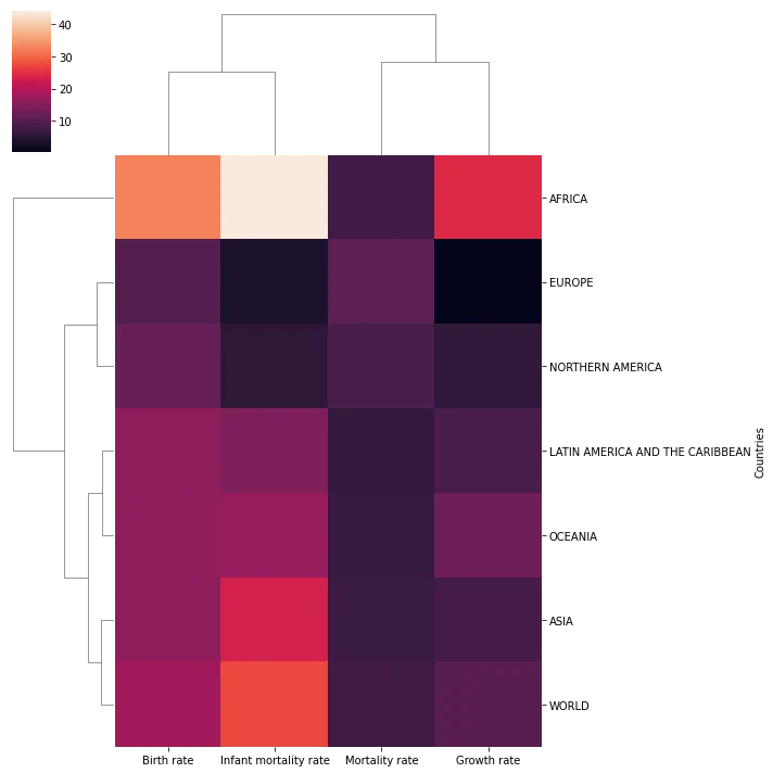
sns.clustermap(rates,col_cluster=False)<seaborn.matrix.ClusterGrid at 0x158e235c9c8>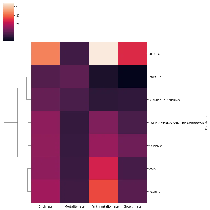
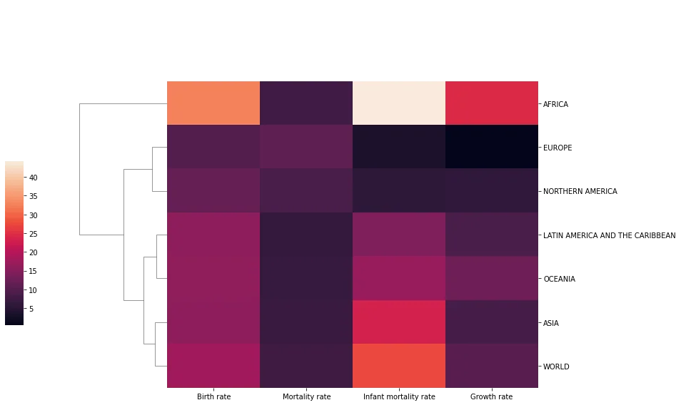
sns.clustermap(rates,col_cluster=False,figsize=(12,8),cbar_pos=(-0.1, .2, .03, .4))<seaborn.matrix.ClusterGrid at 0x158e2ffc848>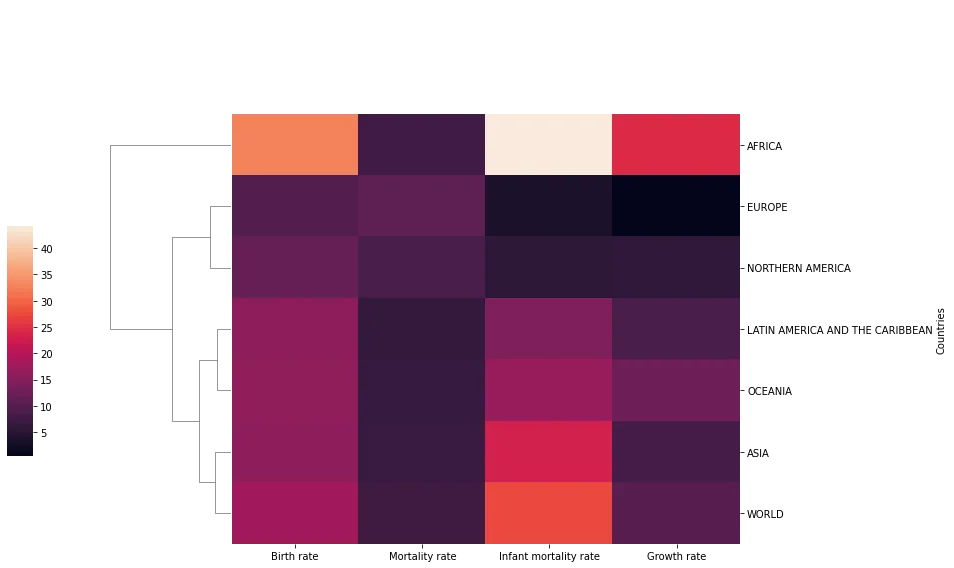
rates.index.set_names('',inplace=True)ratesBirth rate
Mortality rate
Infant mortality rate
Growth rate
AFRICA34 more lines
32.577
7.837
44.215
24.40
ASIA
15.796
7.030
23.185
8.44
EUROPE
10.118
11.163
3.750
0.38
LATIN AMERICA AND THE CARIBBEAN
15.886
6.444
14.570
8.89
NORTHERN AMERICA
11.780
8.833
5.563
6.11
OCEANIA
16.235
6.788
16.939
12.79
WORLD
17.963
7.601
27.492
10.36# Recall you can always edit the DF before seaborn
sns.clustermap(rates,col_cluster=False,figsize=(12,8),cbar_pos=(-0.1, .2, .03, .4))<seaborn.matrix.ClusterGrid at 0x158e354b508>