Categorical Plots - Statistical Estimation within Categories
Often we have categorical data, meaning the data is in distinct groupings, such as Countries or Companies. There is no country value "between" USA and France and there is no company value "between" Google and Apple, unlike continuous data where we know values can exist between data points, such as age or price.
To begin with categorical plots, we'll focus on statistical estimation within categories. Basically this means we will visually report back some statistic (such as mean or count) in a plot. We already know how to get this data with pandas, but often its easier to understand the data if we plot this.
Imports
The Data
df = pd.read_csv("dm_office_sales.csv")df.head()division
level of education
training level
work experience
salary36 more lines
sales
0
printers
some college
2
6
91684
372302
1
printers
associate's degree
2
10
119679
495660
2
peripherals
high school
0
9
82045
320453
3
office supplies
associate's degree
2
5
92949
377148
4
office supplies
high school
1
5
71280
312802
Countplot()
A simple plot, it merely shows the total count of rows per category.
plt.figure(figsize=(10,4),dpi=200)
sns.countplot(x='division',data=df)<AxesSubplot:xlabel='division', ylabel='count'>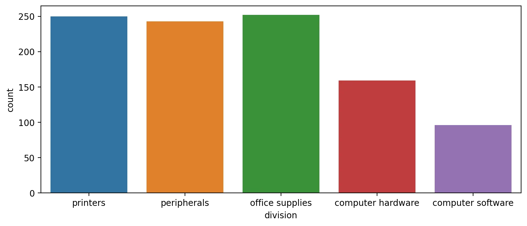
plt.figure(figsize=(10,4),dpi=200)
sns.countplot(x='level of education',data=df)<AxesSubplot:xlabel='level of education', ylabel='count'>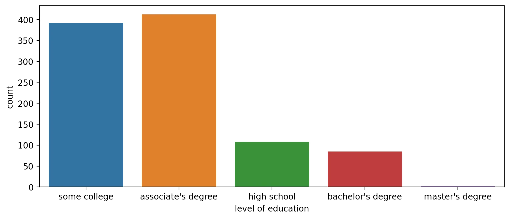
Breakdown within another category with 'hue'
plt.figure(figsize=(10,4),dpi=200)
sns.countplot(x='level of education',data=df,hue='training level')<AxesSubplot:xlabel='level of education', ylabel='count'>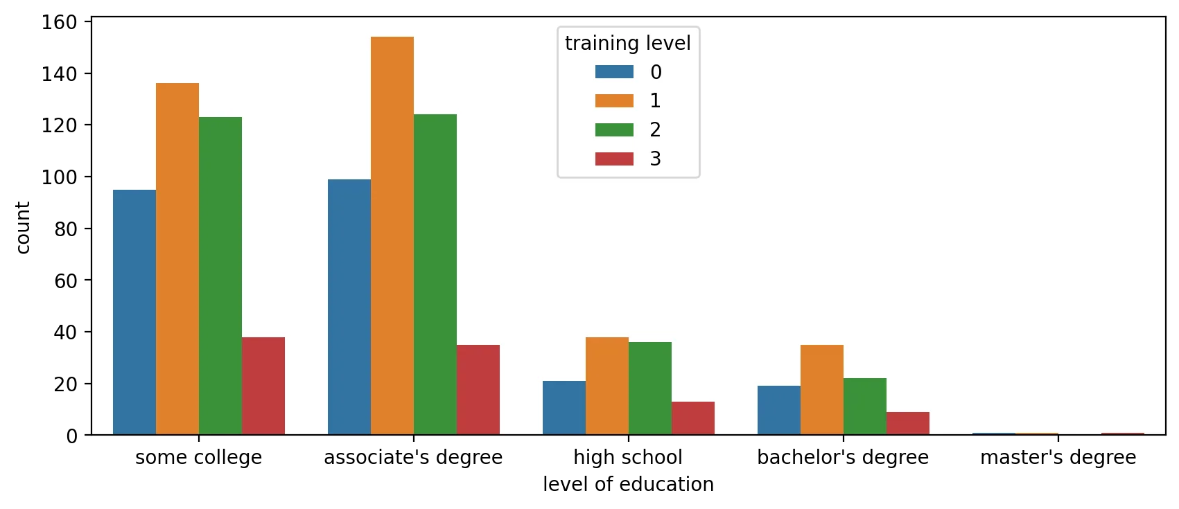
NOTE: You can always edit the palette to your liking to any matplotlib colormap
plt.figure(figsize=(10,4),dpi=200)
sns.countplot(x='level of education',data=df,hue='training level',palette='Set1')<AxesSubplot:xlabel='level of education', ylabel='count'>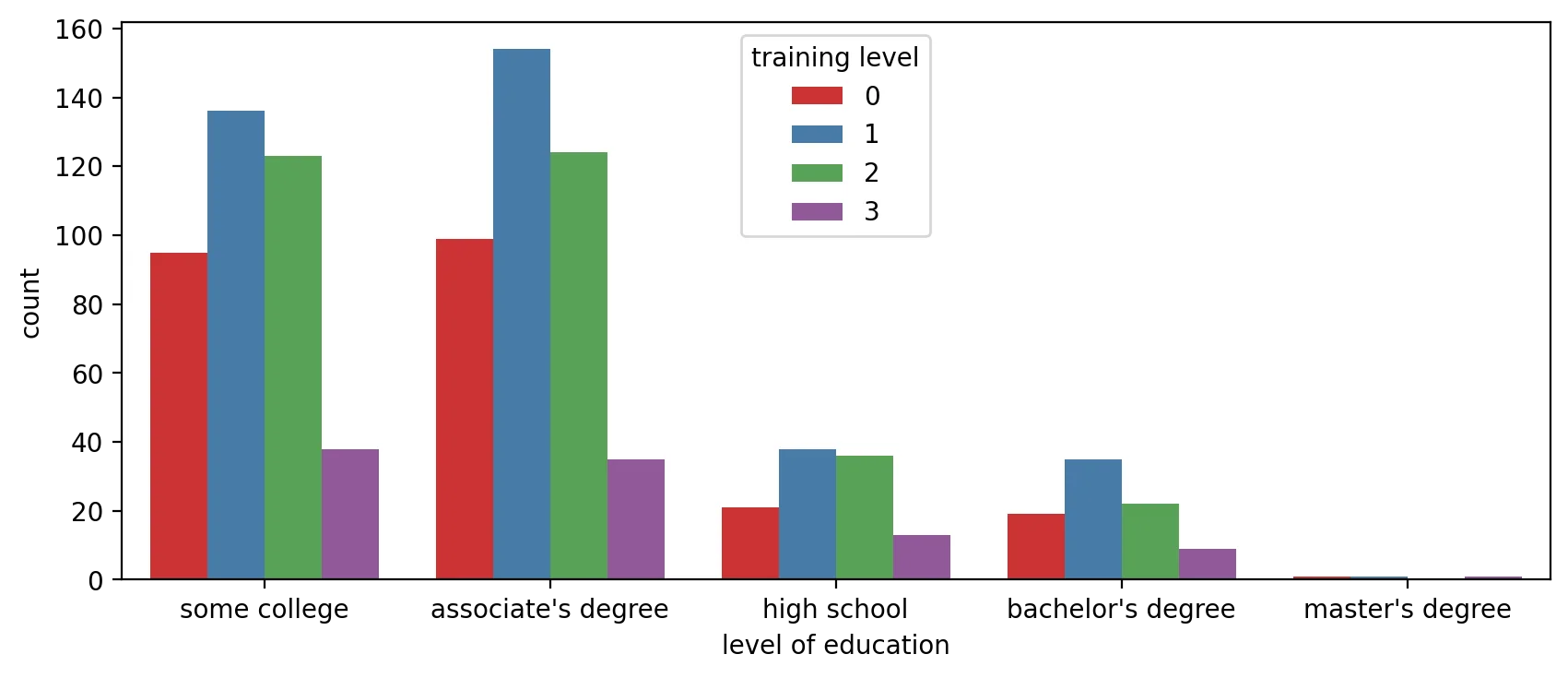
plt.figure(figsize=(10,4),dpi=200)
# Paired would be a good choice if there was a distinct jump from 0 and 1 to 2 and 3
sns.countplot(x='level of education',data=df,hue='training level',palette='Paired')<AxesSubplot:xlabel='level of education', ylabel='count'>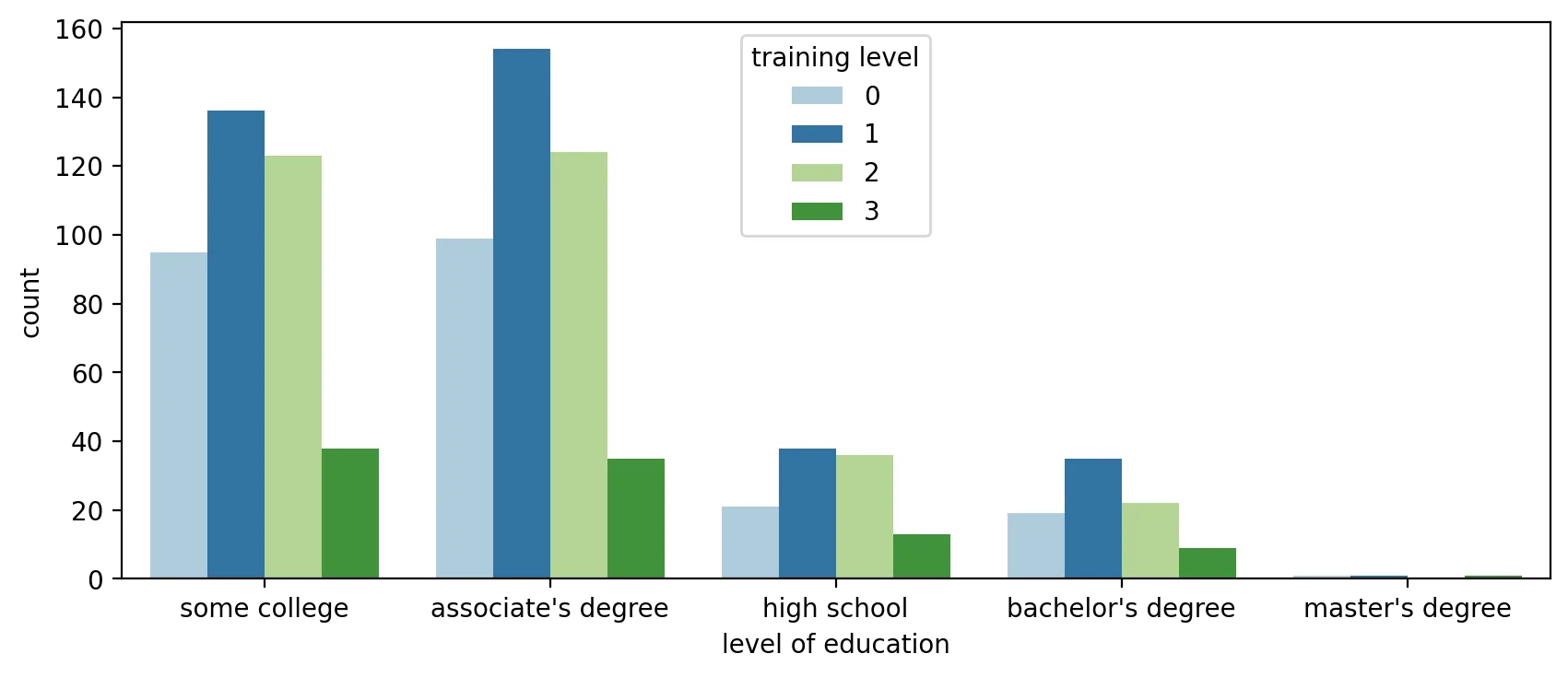
barplot()
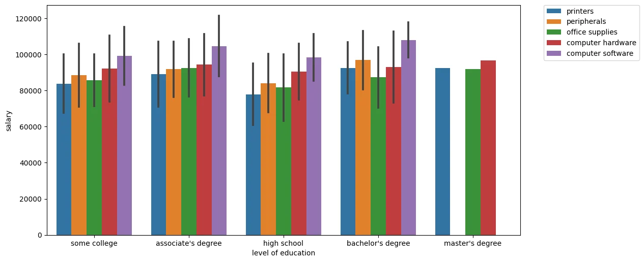
So far we've seen the y axis default to a count (similar to a .groupby(x_axis).count() call in pandas). We can expand our visualizations by specifying a specific continuous feature for the y-axis. Keep in mind, you should be careful with these plots, as they may imply a relationship continuity along the y axis where there is none.
plt.figure(figsize=(10,6),dpi=200)
# By default barplot() will show the mean
# Information on the black bar: https://stackoverflow.com/questions/58362473/what-does-black-lines-on-a-seaborn-barplot-mean
sns.barplot(x='level of education',y='salary',data=df,estimator=np.mean,ci='sd')<AxesSubplot:xlabel='level of education', ylabel='salary'>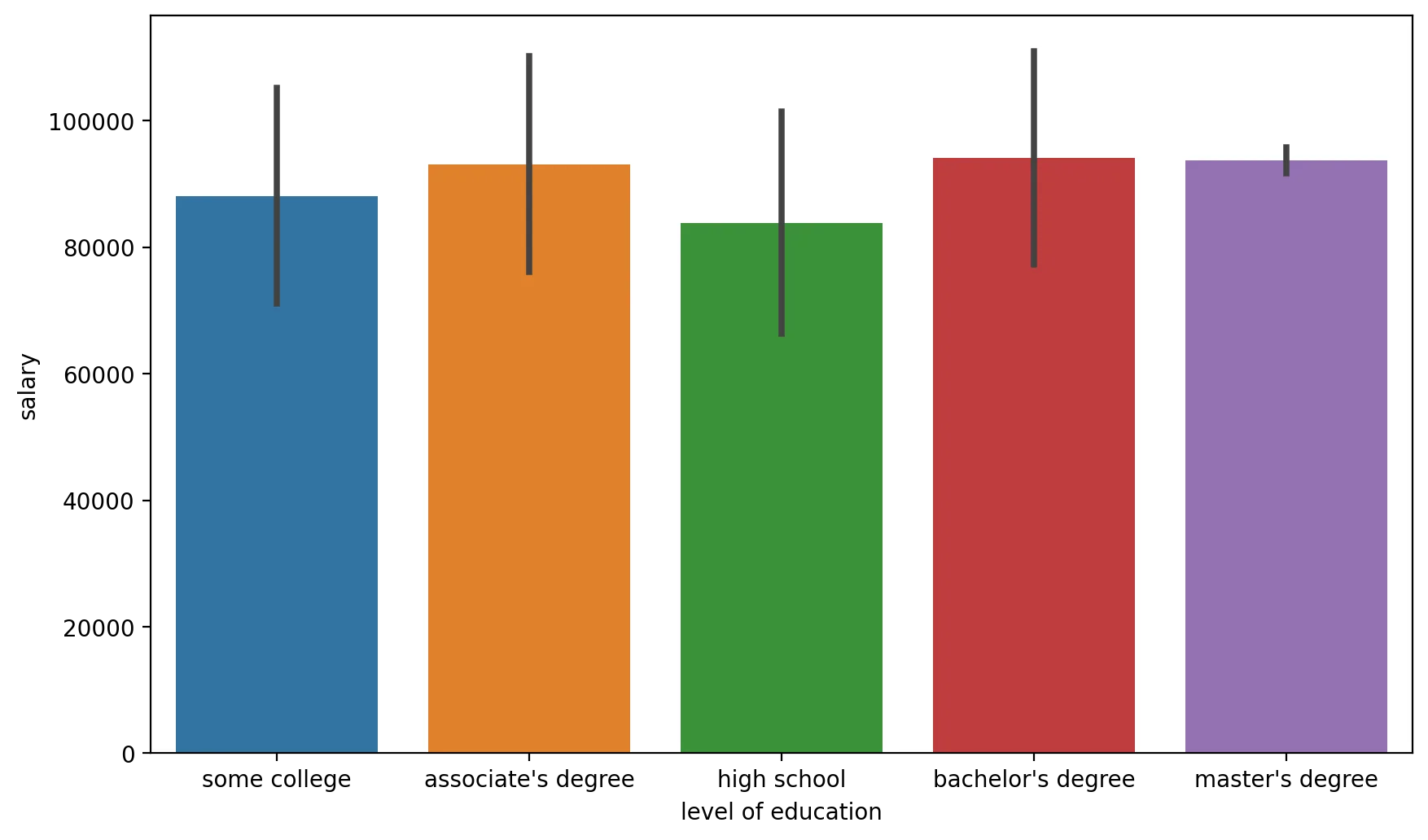
plt.figure(figsize=(12,6))
sns.barplot(x='level of education',y='salary',data=df,estimator=np.mean,ci='sd',hue='division')<AxesSubplot:xlabel='level of education', ylabel='salary'>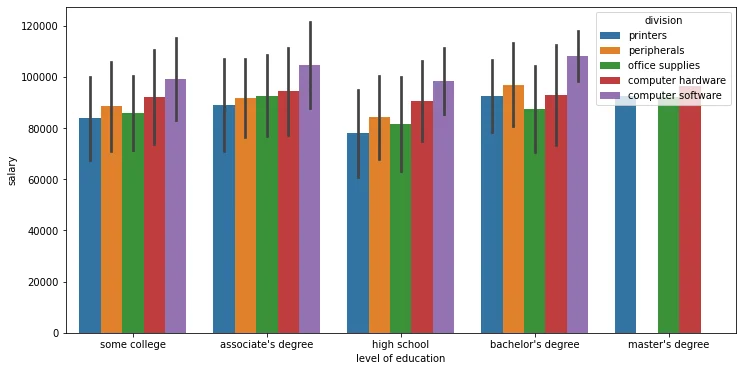
plt.figure(figsize=(12,6),dpi=100)

# https://stackoverflow.com/questions/30490740/move-legend-outside-figure-in-seaborn-tsplot
sns.barplot(x='level of education',y='salary',data=df,estimator=np.mean,ci='sd',hue='division')

plt.legend(bbox_to_anchor=(1.05, 1))<matplotlib.legend.Legend at 0x21fa0b503c8>