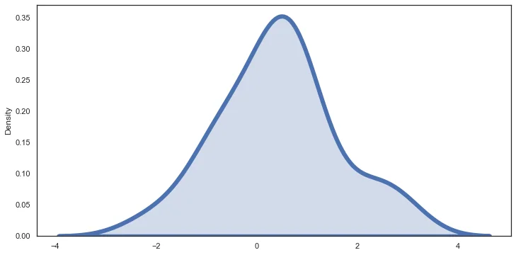
01-Distribution-Plots | Driptanil Datta

Distributions

There are many ways to display the distributions of a feature. In this notebook we explore 3 related plots for displaying a distribution, the rugplot , the distplot (histogram), and kdeplot.

IMPORTANT NOTE!

DO NOT WORRY IF YOUR PLOTS STYLING APPEARS SLIGHTLY DIFFERENT, WE WILL SHOW YOU HOW TO EDIT THE COLOR AND STYLE OF THE PLOTS LATER ON!

Data

We'll use some generated data from: http://roycekimmons.com/tools/generated_data

python

df = pd.read_csv("dm_office_sales.csv")

python

df.head()

Out · table

division
level of education
training level
work experience
salary

36 more lines

sales
0
printers
some college
2
6
91684
372302
1
printers
associate's degree
2
10
119679
495660
2
peripherals
high school
0
9
82045
320453
3
office supplies
associate's degree
2
5
92949
377148
4
office supplies
high school
1
5
71280
312802

python

df.info()

Out · stdout

<class 'pandas.core.frame.DataFrame'>
RangeIndex: 1000 entries, 0 to 999
Data columns (total 6 columns):
 #   Column              Non-Null Count  Dtype 
---  ------              --------------  -----

8 more lines

 0   division            1000 non-null   object
 1   level of education  1000 non-null   object
 2   training level      1000 non-null   int64 
 3   work experience     1000 non-null   int64 
 4   salary              1000 non-null   int64 
 5   sales               1000 non-null   int64 
dtypes: int64(4), object(2)
memory usage: 47.0+ KB

Rugplot

Very simple plot that puts down one mark per data point. This plot needs the single array passed in directly. We won't use it too much since its not very clarifying for large data sets.

python

# The y axis doesn't really represent anything
# X axis is just a stick per data point
sns.rugplot(x='salary',data=df)

Out · result

<AxesSubplot:xlabel='salary'>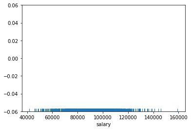

python

sns.rugplot(x='salary',data=df,height=0.5)

Out · result

<AxesSubplot:xlabel='salary'>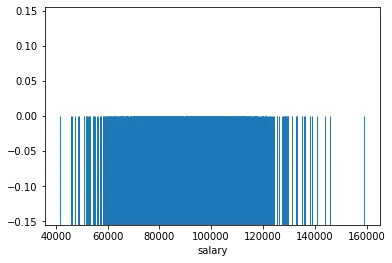

displot() and histplot()

The rugplot itself is not very informative for larger data sets distribution around the mean since so many ticks makes it hard to distinguish one tick from another. Instead we should count the number of tick marks per some segment of the x axis, then construct a histogram from this.

The displot is a plot type that can show you the distribution of a single feature. It is a histogram with the option of adding a "KDE" plot (Kernel Density Estimation) on top of the histogram. Let's explore its use cases and syntax.

python

sns.displot(data=df,x='salary',kde=True)

Out · result

<seaborn.axisgrid.FacetGrid at 0x26e5cd14cc8>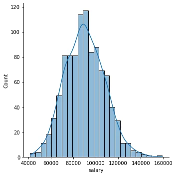

Focusing on the Histogram

python

sns.displot(data=df,x='salary')

Out · result

<seaborn.axisgrid.FacetGrid at 0x26e5ce18748>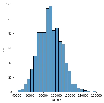

python

sns.histplot(data=df,x='salary')

Out · result

<AxesSubplot:xlabel='salary', ylabel='Count'>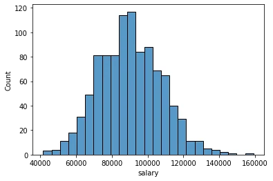

Number of Bins

python

sns.histplot(data=df,x='salary',bins=10)

Out · result

<AxesSubplot:xlabel='salary', ylabel='Count'>

python

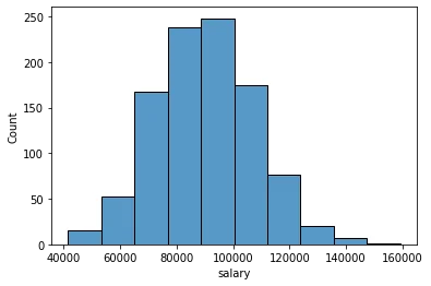
sns.histplot(data=df,x='salary',bins=100)

Out · result

<AxesSubplot:xlabel='salary', ylabel='Count'>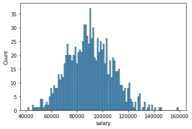

Adding in a grid and styles

You can reset to a different default style: one of {darkgrid, whitegrid, dark, white, ticks}.

In a later notebook and lecture we will cover custom styling in a lot more detail.

python

sns.set(style='darkgrid')
sns.histplot(data=df,x='salary',bins=100)

Out · result

<AxesSubplot:xlabel='salary', ylabel='Count'>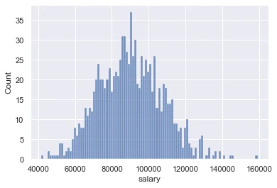

python

sns.set(style='white')
sns.histplot(data=df,x='salary',bins=100)

Out · result

<AxesSubplot:xlabel='salary', ylabel='Count'>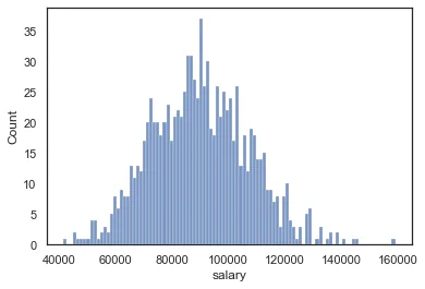

Adding in keywords from matplotlib

Seaborn plots can accept keyword arguments directly from the matplotlib code that seaborn uses. Keep in mind, not every seaborn plot can accept all matplotlib arguments, but the main styling parameters we've discussed are available.

python

sns.displot(data=df,x='salary',bins=20,kde=False,
            color='red',edgecolor='black',lw=4,ls='--')

Out · result

<seaborn.axisgrid.FacetGrid at 0x26e5d449f48>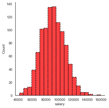

The Kernel Density Estimation Plot

Note: Review the video for full detailed explanation.

The KDE plot maps an estimate of a probability density function of a random variable. Kernel density estimation is a fundamental data smoothing problem where inferences about the population are made, based on a finite data sample.

Let's build out a simple example:

python

np.random.seed(42)

# randint should be uniform, each age has the same chance of being chosen
# note: in reality ages are almost never uniformally distributed, but this is just an example
sample_ages = np.random.randint(0,100,200)

python

sample_ages

Out · result

array([51, 92, 14, 71, 60, 20, 82, 86, 74, 74, 87, 99, 23,  2, 21, 52,  1,
       87, 29, 37,  1, 63, 59, 20, 32, 75, 57, 21, 88, 48, 90, 58, 41, 91,
       59, 79, 14, 61, 61, 46, 61, 50, 54, 63,  2, 50,  6, 20, 72, 38, 17,
        3, 88, 59, 13,  8, 89, 52,  1, 83, 91, 59, 70, 43,  7, 46, 34, 77,
       80, 35, 49,  3,  1,  5, 53,  3, 53, 92, 62, 17, 89, 43, 33, 73, 61,

7 more lines

       99, 13, 94, 47, 14, 71, 77, 86, 61, 39, 84, 79, 81, 52, 23, 25, 88,
       59, 40, 28, 14, 44, 64, 88, 70,  8, 87,  0,  7, 87, 62, 10, 80,  7,
       34, 34, 32,  4, 40, 27,  6, 72, 71, 11, 33, 32, 47, 22, 61, 87, 36,
       98, 43, 85, 90, 34, 64, 98, 46, 77,  2,  0,  4, 89, 13, 26,  8, 78,
       14, 89, 41, 76, 50, 62, 95, 51, 95,  3, 93, 22, 14, 42, 28, 35, 12,
       31, 70, 58, 85, 27, 65, 41, 44, 61, 56,  5, 27, 27, 43, 83, 29, 61,
       74, 91, 88, 61, 96,  0, 26, 61, 76,  2, 69, 71, 26])

python

sample_ages = pd.DataFrame(sample_ages,columns=["age"])

python

sample_ages.head()

Out · table

age
0
51
1
92

6 more lines

python

sns.rugplot(data=sample_ages,x='age')

Out · result

<AxesSubplot:xlabel='age'>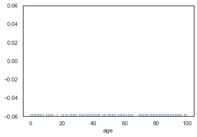

python

plt.figure(figsize=(12,8))
sns.displot(data=sample_ages,x='age',bins=10,rug=True)

Out · result

<seaborn.axisgrid.FacetGrid at 0x26e5ec12688>

Out · result

<Figure size 864x576 with 0 Axes>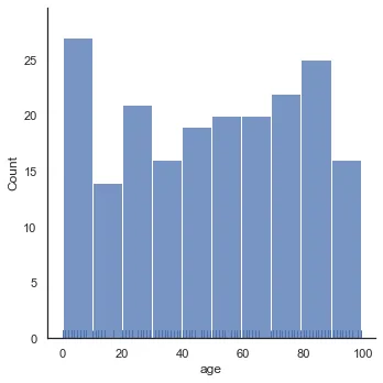

python

plt.figure(figsize=(12,8))
sns.displot(data=sample_ages,x='age',bins=10,rug=True,kde=True)

Out · result

<seaborn.axisgrid.FacetGrid at 0x26e5ec41f08>

Out · result

<Figure size 864x576 with 0 Axes>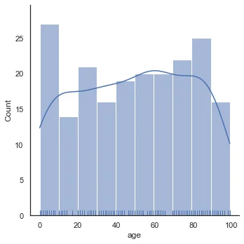

python

sns.kdeplot(data=sample_ages,x='age')

Out · result

<AxesSubplot:xlabel='age', ylabel='Density'>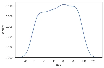

Cut Off KDE

We could cut off the KDE if we know our data has hard limits (no one can be a negative age and no one in the population can be older than 100 for some reason)

python

# plt.figure(figsize=(12,8))
sns.kdeplot(data=sample_ages,x='age',clip=[0,100])

Out · result

<AxesSubplot:xlabel='age', ylabel='Density'>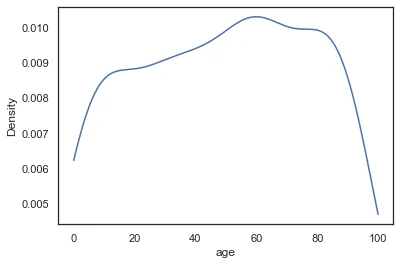

Bandwidth

As explained in the video, the KDE is constructed through the summation of the kernel (most commonly Gaussian), we can effect the bandwith of this kernel to make the KDE more "sensitive" to the data. Notice how with a smaller bandwith, the kernels don't stretch so wide, meaning we don't need the cut-off anymore. This is analagous to increasing the number of bins in a histogram (making the actual bins narrower).

python

sns.kdeplot(data=sample_ages,x='age',bw_adjust=0.1)

Out · result

<AxesSubplot:xlabel='age', ylabel='Density'>

python

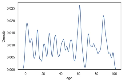
sns.kdeplot(data=sample_ages,x='age',bw_adjust=0.5)

Out · result

<AxesSubplot:xlabel='age', ylabel='Density'>

python

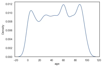
sns.kdeplot(data=sample_ages,x='age',bw_adjust=1)

Out · result

<AxesSubplot:xlabel='age', ylabel='Density'>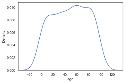

Basic Styling

There are a few basic styling calls directly availble in a KDE.

python

sns.kdeplot(data=sample_ages,x='age',bw_adjust=0.5,shade=True,color='red')

Out · result

<AxesSubplot:xlabel='age', ylabel='Density'>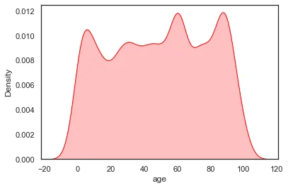

2 Dimensional KDE Plots

We will cover these in more detail later, but just keep in mind you could compare two continuous features and create a 2d KDE plot showing there distributions with the same kdeplot() call. Don't worry about this now, since we will cover it in more detail later when we talk about comparing 2 features against each other in a plot call.

python

random_data = pd.DataFrame(np.random.normal(0,1,size=(100,2)),columns=['x','y'])

python

random_data

Out · table

x
y
0
-1.415371
-0.420645

31 more lines

1
-0.342715
-0.802277
2
-0.161286
0.404051
3
1.886186
0.174578
4
0.257550
-0.074446
...
...
...
95
-0.208122
-0.493001
96
-0.589365
0.849602
97
0.357015
-0.692910
98
0.899600
0.307300
99
0.812862
0.629629
100 rows × 2 columns

python

sns.kdeplot(data=random_data,x='x',y='y')

Out · result

<AxesSubplot:xlabel='x', ylabel='y'>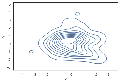

Bonus Code for Visualizations from Video Lecture

Below is the code used to create the visualizations shown in the video lecture for an explanation of a KDE plot. We will not cover this code in further detail, since it was only used for the creation of the slides shown in the video.

python

from scipy import stats

Data

python

np.random.seed(101)
x = np.random.normal(0, 1, size=20)

python

plt.figure(figsize=(8,4),dpi=200)
sns.rugplot(x, color="darkblue", linewidth=4)

Out · result

<AxesSubplot:>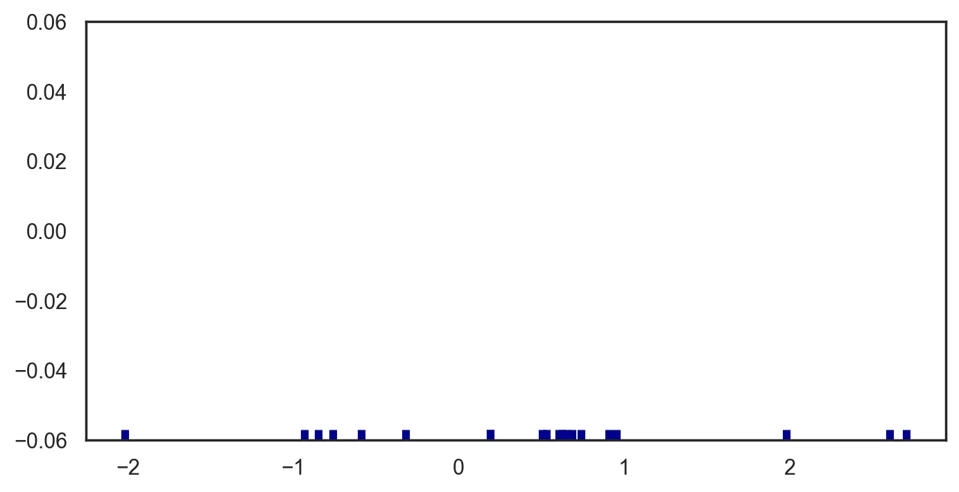

python

plt.figure(figsize=(8,4),dpi=200)
bandwidth = x.std() * x.size ** (-0.001)
support = np.linspace(-5, 5, 100)

kernels = []

plt.figure(figsize=(12,6))

for x_i in x:

    kernel = stats.norm(x_i, bandwidth).pdf(support)
    kernels.append(kernel)
    plt.plot(support, kernel, color="lightblue")

sns.rugplot(x, color="darkblue", linewidth=4);

Out · result

<Figure size 1600x800 with 0 Axes>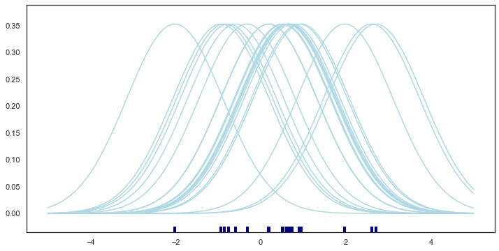

python

plt.figure(figsize=(8,4),dpi=200)
from scipy.integrate import trapz
plt.figure(figsize=(12,6))
density = np.sum(kernels, axis=0)
density /= trapz(density, support)
plt.plot(support, density);
sns.rugplot(x, color="darkblue", linewidth=4);

Out · result

<Figure size 1600x800 with 0 Axes>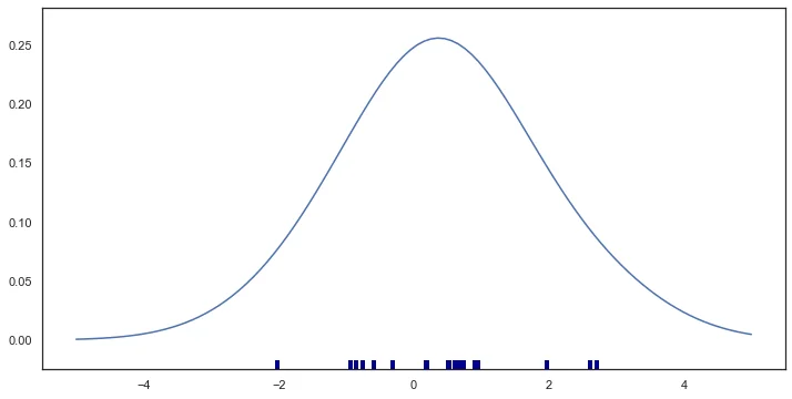

python

plt.figure(figsize=(8,4),dpi=200)
bandwidth = x.std() * x.size ** (-0.001)
support = np.linspace(-5, 5, 100)

kernels = []

plt.figure(figsize=(12,6))

for x_i in x:

    kernel = stats.norm(x_i, bandwidth).pdf(support)
    kernels.append(kernel)
#     plt.plot(support, kernel, color="lightblue")

# sns.rugplot(x, color="darkblue", linewidth=4);
sns.kdeplot(x,linewidth=6,shade=True)

Out · result

<AxesSubplot:ylabel='Density'>

Out · result

<Figure size 1600x800 with 0 Axes>