03-Categorical-Plots-Distributions

Categorical Plots - Distribution within Categories

So far we've seen how to apply a statistical estimation (like mean or count) to categories and compare them to one another. Let's now explore how to visualize the distribution within categories. We already know about distplot() which allows to view the distribution of a single feature, now we will break down that same distribution per category.

Imports

The Data

df = pd.read_csv("StudentsPerformance.csv")

df.head()

gender
race/ethnicity
parental level of education
lunch
test preparation course

math score
reading score
writing score
0
female
group B
bachelor's degree
standard
none
72
72
74
1
female
group C
some college
standard
completed
69
90
88
2
female
group B
master's degree
standard
none
90
95
93
3
male
group A
associate's degree
free/reduced
none
47
57
44
4
male
group C
some college
standard
none
76
78
75

Boxplot

As described in the video, a boxplot display distribution through the use of quartiles and an IQR for outliers.

plt.figure(figsize=(12,6))
sns.boxplot(x='parental level of education',y='math score',data=df)

<AxesSubplot:xlabel='parental level of education', ylabel='math score'>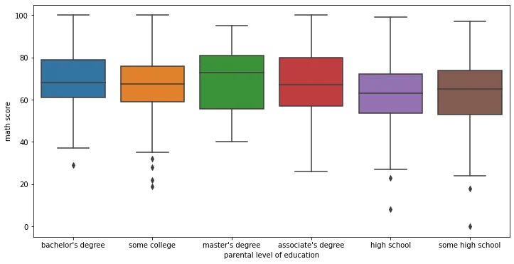

Adding hue for further segmentation

plt.figure(figsize=(12,6))
sns.boxplot(x='parental level of education',y='math score',data=df,hue='gender')

# Optional move the legend outside
plt.legend(bbox_to_anchor=(1.05, 1), loc=2, borderaxespad=0.)

<matplotlib.legend.Legend at 0x215583a7e08>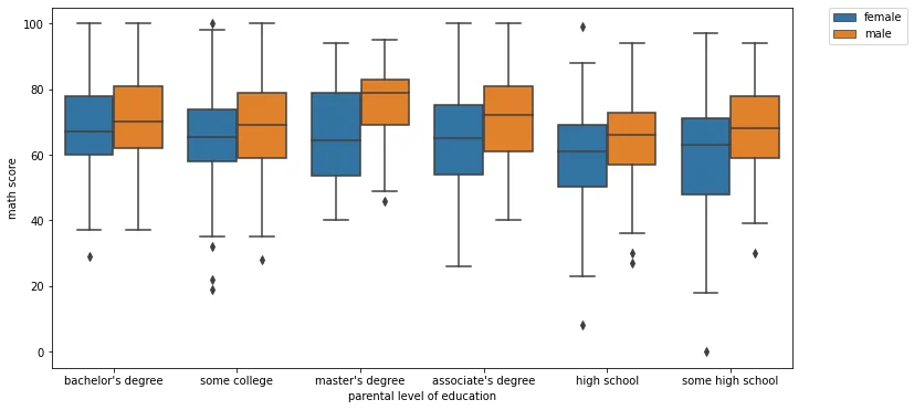

Boxplot Styling Parameters

Orientation

# NOTICE HOW WE HAVE TO SWITCH X AND Y FOR THE ORIENTATION TO MAKE SENSE!
sns.boxplot(x='math score',y='parental level of education',data=df,orient='h')

<AxesSubplot:xlabel='math score', ylabel='parental level of education'>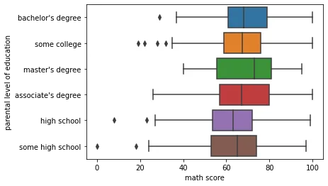

Width

plt.figure(figsize=(12,6))
sns.boxplot(x='parental level of education',y='math score',data=df,hue='gender',width=0.3)

<AxesSubplot:xlabel='parental level of education', ylabel='math score'>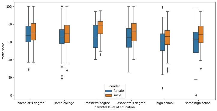

Violinplot

A violin plot plays a similar role as a box and whisker plot. It shows the distribution of quantitative data across several levels of one (or more) categorical variables such that those distributions can be compared. Unlike a box plot, in which all of the plot components correspond to actual datapoints, the violin plot features a kernel density estimation of the underlying distribution.

plt.figure(figsize=(12,6))
sns.violinplot(x='parental level of education',y='math score',data=df)

<AxesSubplot:xlabel='parental level of education', ylabel='math score'>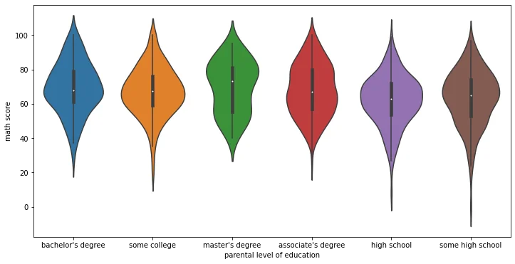

plt.figure(figsize=(12,6))
sns.violinplot(x='parental level of education',y='math score',data=df,hue='gender')

<AxesSubplot:xlabel='parental level of education', ylabel='math score'>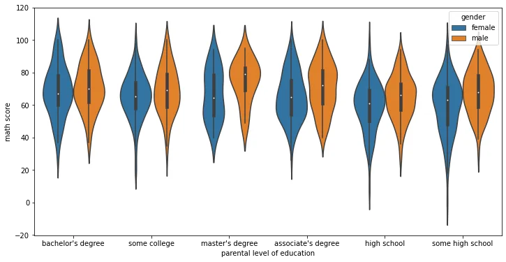

Violinplot Parameters

split

When using hue nesting with a variable that takes two levels, setting split to True will draw half of a violin for each level. This can make it easier to directly compare the distributions.

plt.figure(figsize=(12,6))
sns.violinplot(x='parental level of education',y='math score',data=df,hue='gender',split=True)

<AxesSubplot:xlabel='parental level of education', ylabel='math score'>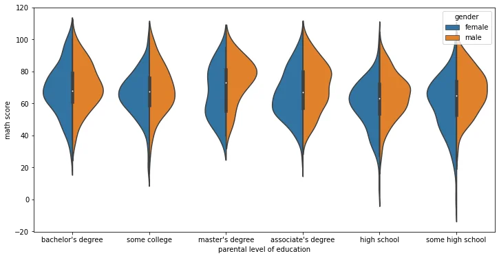

inner

Representation of the datapoints in the violin interior. If box, draw a miniature boxplot. If quartiles, draw the quartiles of the distribution. If point or stick, show each underlying datapoint. Using None will draw unadorned violins.

plt.figure(figsize=(12,6))
sns.violinplot(x='parental level of education',y='math score',data=df,inner=None)

<AxesSubplot:xlabel='parental level of education', ylabel='math score'>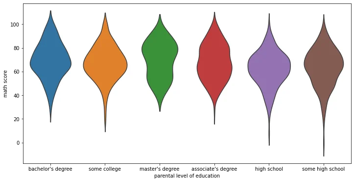

plt.figure(figsize=(12,6))
sns.violinplot(x='parental level of education',y='math score',data=df,inner='box')

<AxesSubplot:xlabel='parental level of education', ylabel='math score'>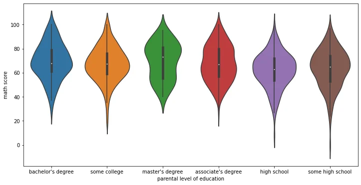

plt.figure(figsize=(12,6))
sns.violinplot(x='parental level of education',y='math score',data=df,inner='quartile')

<AxesSubplot:xlabel='parental level of education', ylabel='math score'>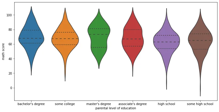

plt.figure(figsize=(12,6))
sns.violinplot(x='parental level of education',y='math score',data=df,inner='stick')

<AxesSubplot:xlabel='parental level of education', ylabel='math score'>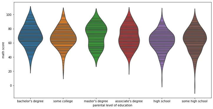

orientation

# Simply switch the continuous variable to y and the categorical to x
sns.violinplot(x='math score',y='parental level of education',data=df,)

<AxesSubplot:xlabel='math score', ylabel='parental level of education'>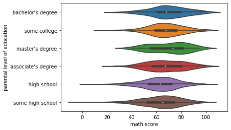

bandwidth

Similar to bandwidth argument for kdeplot

plt.figure(figsize=(12,6))
sns.violinplot(x='parental level of education',y='math score',data=df,bw=0.1)

<AxesSubplot:xlabel='parental level of education', ylabel='math score'>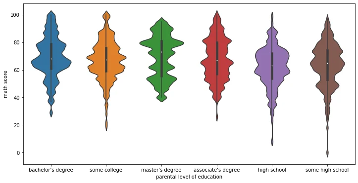

Advanced Plots

We can use a boxenplot and swarmplot to achieve the same effect as the boxplot and violinplot, but with slightly more information included. Be careful when using these plots, as they often require you to educate the viewer with how the plot is actually constructed. Only use these if you are sure your audience will understand the visualization.

df.head()

gender
race/ethnicity
parental level of education
lunch
test preparation course

math score
reading score
writing score
0
female
group B
bachelor's degree
standard
none
72
72
74
1
female
group C
some college
standard
completed
69
90
88
2
female
group B
master's degree
standard
none
90
95
93
3
male
group A
associate's degree
free/reduced
none
47
57
44
4
male
group C
some college
standard
none
76
78
75

swarmplot

sns.swarmplot(x='math score',data=df)

c:\users\marcial\anaconda3\envs\ml_master\lib\site-packages\seaborn\categorical.py:1296: UserWarning: 15.8% of the points cannot be placed; you may want to decrease the size of the markers or use stripplot.
  warnings.warn(msg, UserWarning)

<AxesSubplot:xlabel='math score'>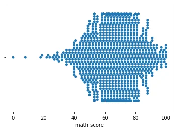

sns.swarmplot(x='math score',data=df,size=2)

<AxesSubplot:xlabel='math score'>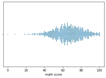

sns.swarmplot(x='math score',y='race/ethnicity',data=df,size=3)

<AxesSubplot:xlabel='math score', ylabel='race/ethnicity'>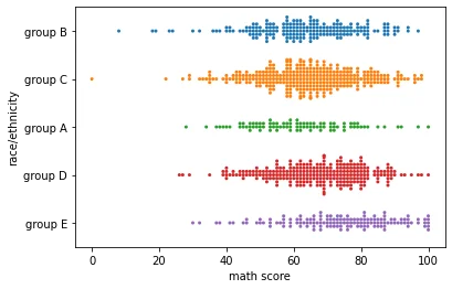

sns.swarmplot(x='race/ethnicity',y='math score',data=df,size=3)

<AxesSubplot:xlabel='race/ethnicity', ylabel='math score'>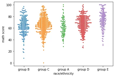

plt.figure(figsize=(12,6))
sns.swarmplot(x='race/ethnicity',y='math score',data=df,hue='gender')

<AxesSubplot:xlabel='race/ethnicity', ylabel='math score'>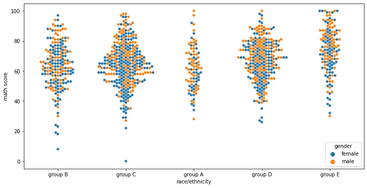

plt.figure(figsize=(12,6))
sns.swarmplot(x='race/ethnicity',y='math score',data=df,hue='gender',dodge=True)

c:\users\marcial\anaconda3\envs\ml_master\lib\site-packages\seaborn\categorical.py:1296: UserWarning: 6.7% of the points cannot be placed; you may want to decrease the size of the markers or use stripplot.
  warnings.warn(msg, UserWarning)

<AxesSubplot:xlabel='race/ethnicity', ylabel='math score'>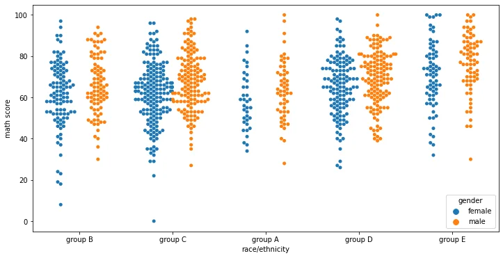

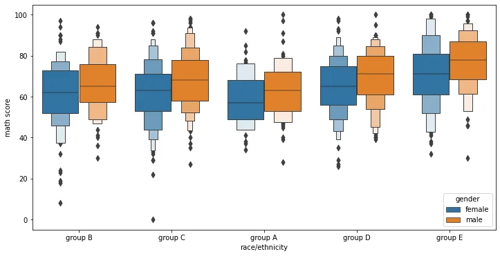
boxenplot (letter-value plot)

Official Paper on this plot: https://vita.had.co.nz/papers/letter-value-plot.html

This style of plot was originally named a “letter value” plot because it shows a large number of quantiles that are defined as “letter values”. It is similar to a box plot in plotting a nonparametric representation of a distribution in which all features correspond to actual observations. By plotting more quantiles, it provides more information about the shape of the distribution, particularly in the tails.

sns.boxenplot(x='math score',y='race/ethnicity',data=df)

<AxesSubplot:xlabel='math score', ylabel='race/ethnicity'>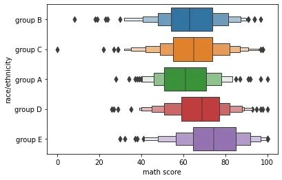

sns.boxenplot(x='race/ethnicity',y='math score',data=df)

<AxesSubplot:xlabel='race/ethnicity', ylabel='math score'>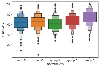

plt.figure(figsize=(12,6))
sns.boxenplot(x='race/ethnicity',y='math score',data=df,hue='gender')

<AxesSubplot:xlabel='race/ethnicity', ylabel='math score'>