7. Dot Product Geometry

The Dot Product: Geometric Perspective

Historically, the dot product was developed through two different lenses: the algebraic approach (multiplying elements and summing them) and the geometric approach (projecting vectors onto one another in space). In this lesson, we explore the geometric definition of the dot product, learn how to calculate angles between vectors in high dimensions, categorize vector relationships based on their signs, and perform the classic proof linking algebra and geometry together.

1. The Geometric Formula

Geometrically, the dot product between two column vectors $\mathbf{a}$ and $\mathbf{b}$ is defined as the product of their magnitudes (lengths) scaled by the cosine of the angle $\theta$ between them:

Where:

• $\|\mathbf{a}\|$ and $\|\mathbf{b}\|$ represent the vector lengths.
• $\theta$ is the angle between the two vectors in space.

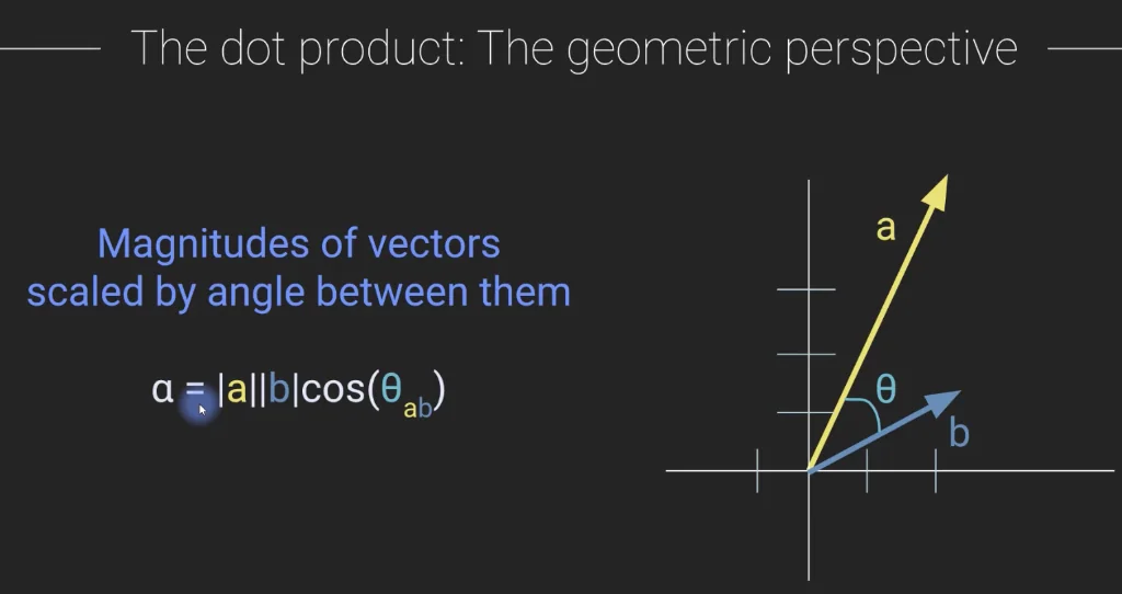
Flexible Notation Conventions: In mathematical literature, you will see length represented with either double bars ($\|\mathbf{a}\|$) or single bars ($|\mathbf{a}|$). Do not get thrown off by formatting variations; they represent the exact same concept of vector magnitude.

2. Computing the Angle Between Vectors

We can rearrange the geometric formula to solve for the angle $\theta$. This provides a universal equation to find the spatial angle between any two vectors:

1. Divide by the magnitudes: $$\cos(\theta) = \frac{\mathbf{a}^{\text{T}}\mathbf{b}}{\|\mathbf{a}\|\|\mathbf{b}\|}$$
2. Apply the inverse cosine ($\arccos$): $$\theta = \arccos\left( \frac{\mathbf{a}^{\text{T}}\mathbf{b}}{\|\mathbf{a}\|\|\mathbf{b}\|} \right)$$

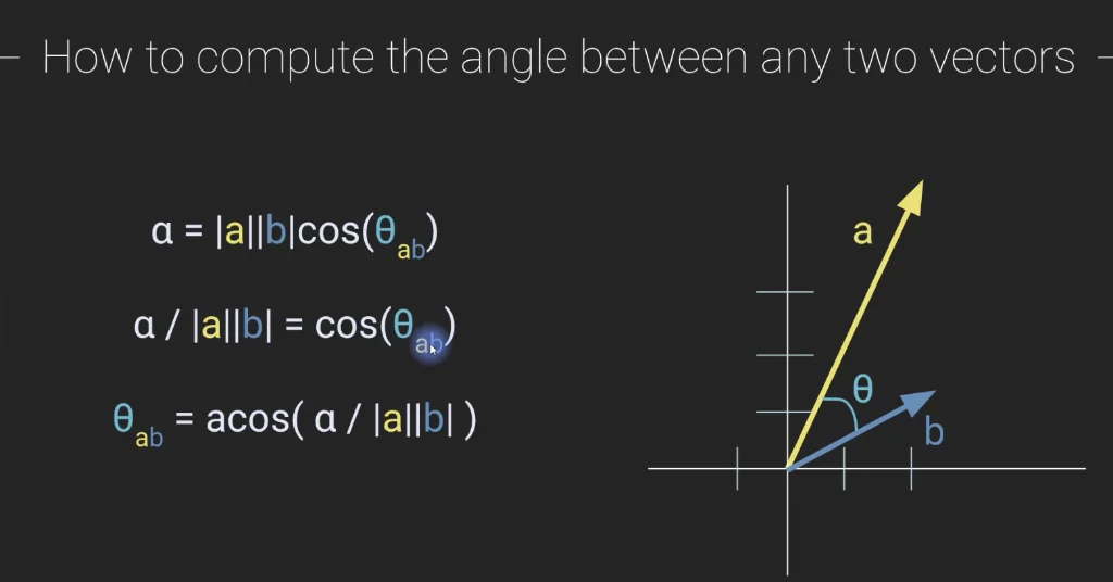
This formula is incredibly powerful. Although derived from a 2D coordinates system, it works for vectors of any arbitrary dimensionality $n \in \mathbb{R}^n$. Even though we cannot visualize a 10-dimensional space, we can calculate the exact angle between two 10D vectors instantly using this formula.

3. Dot Product Sign Categories

Because vector magnitudes $\|\mathbf{a}\|$ and $\|\mathbf{b}\|$ are strictly non-negative, the sign of the dot product is is determined entirely by the cosine of the angle $\theta$ between them. This categorizes the spatial relationships between vectors into four key states:

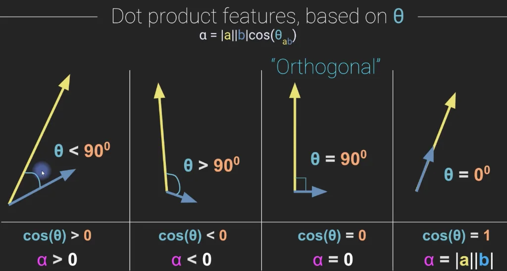
Category 1: Acute Angle ($\theta < 90^\circ$)

• Cosine Value: $\cos(\theta) > 0$
• Dot Product Sign: $\mathbf{a}^{\text{T}}\mathbf{b} > 0$ (Positive)
• Meaning: The vectors point generally in the same direction.

Category 2: Obtuse Angle ($\theta > 90^\circ$)

• Cosine Value: $\cos(\theta) < 0$
• Dot Product Sign: $\mathbf{a}^{\text{T}}\mathbf{b} < 0$ (Negative)
• Meaning: The vectors point generally in opposite directions.

Category 3: Right Angle / Orthogonal ($\theta = 90^\circ$)

• Cosine Value: $\cos(\theta) = 0$
• Dot Product Sign: $\mathbf{a}^{\text{T}}\mathbf{b} = 0$ (Zero)
• Concept (Orthogonality): This is one of the most critical concepts in linear algebra. Two non-zero vectors are orthogonal if and only if their dot product is exactly $0$.

Category 4: Collinear Same Direction ($\theta = 0^\circ$)

• Cosine Value: $\cos(0) = 1$
• Dot Product Sign: $\mathbf{a}^{\text{T}}\mathbf{b} = \|\mathbf{a}\|\|\mathbf{b}\|$
• Self Dot Product: If a vector is dotted with itself ($\mathbf{b} = \mathbf{a}$), the angle is $0$. This yields $\mathbf{a}^{\text{T}}\mathbf{a} = \|\mathbf{a}\|^2$, which algebraically proves why $\|\mathbf{a}\| = \sqrt{\mathbf{a}^{\text{T}}\mathbf{a}}$.

Category 5: Collinear Opposite Direction ($\theta = 180^\circ$)

• Cosine Value: $\cos(180^\circ) = -1$
• Dot Product Sign: $\mathbf{a}^{\text{T}}\mathbf{b} = -\|\mathbf{a}\|\|\mathbf{b}\|$

4. The Equivalence Proof: Algebra vs. Geometry

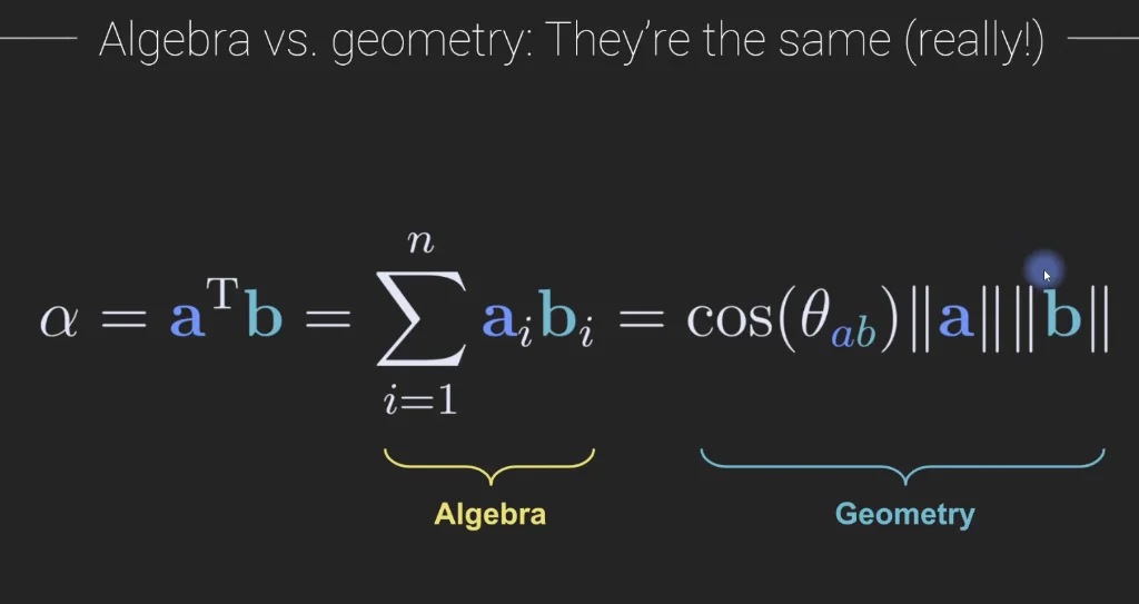
To prove that the algebraic summation formula $\sum \mathbf{a}_i \mathbf{b}_i$ is mathematically identical to the geometric formula $\|\mathbf{a}\|\|\mathbf{b}\|\cos(\theta)$, we rely on the Law of Cosines.

Step 1: Proving the Law of Cosines

Consider a triangle with side lengths $a, b, c$ and angle $\theta$ opposite to side $c$. By dropping a perpendicular height $a_1$ onto side $b$, we split $b$ into two segments $b_2$ and $b_1$:

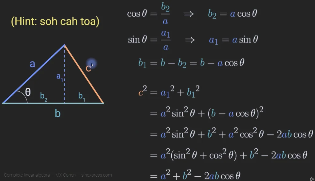
Using basic right-angled trigonometry (Soh-Cah-Toa): $$\cos(\theta) = \frac{b_2}{a} \implies B_2 = a\cos(\theta)$$ $$\sin(\theta) = \frac{a_1}{a} \implies a_1 = a\sin(\theta)$$

The remaining segment $b_1$ is: $$b_1 = b - b_2 = b - a\cos(\theta)$$

Applying the Pythagorean theorem to the right-hand right triangle: $$c^2 = a_1^2 + b_1^2$$ $$c^2 = (a\sin\theta)^2 + (b - a\cos\theta)^2$$ $$c^2 = a^2\sin^2\theta + b^2 - 2ab\cos\theta + a^2\cos^2\theta$$ $$c^2 = a^2(\sin^2\theta + \cos^2\theta) + b^2 - 2ab\cos\theta$$

Using the trigonometric identity $\sin^2\theta + \cos^2\theta = 1$, we get the Law of Cosines: $$c^2 = a^2 + b^2 - 2ab\cos\theta$$

Step 2: Vector Translation

Now, let's represent this triangle using vectors in space. Let the sides of the triangle be defined by vectors $\mathbf{a}$ and $\mathbf{b}$. The third side connecting their tips represents the subtraction vector $\mathbf{a} - \mathbf{b}$.

Applying their lengths into the Law of Cosines: $$\|\mathbf{a} - \mathbf{b}\|^2 = \|\mathbf{a}\|^2 + \|\mathbf{b}\|^2 - 2\|\mathbf{a}\|\|\mathbf{b}\|\cos\theta$$

We also know algebraically that the squared length of any vector is the dot product with itself: $$\|\mathbf{a} - \mathbf{b}\|^2 = (\mathbf{a} - \mathbf{b})^{\text{T}}(\mathbf{a} - \mathbf{b})$$ $$= \mathbf{a}^{\text{T}}\mathbf{a} - \mathbf{a}^{\text{T}}\mathbf{b} - \mathbf{b}^{\text{T}}\mathbf{a} + \mathbf{b}^{\text{T}}\mathbf{b}$$

Since the dot product commutes (which we verify in Python), $\mathbf{b}^{\text{T}}\mathbf{a} = \mathbf{a}^{\text{T}}\mathbf{b}$: $$= \|\mathbf{a}\|^2 + \|\mathbf{b}\|^2 - 2\mathbf{a}^{\text{T}}\mathbf{b}$$

Step 3: Equating the Formulas

Since both expressions represent the exact same squared distance $\|\mathbf{a} - \mathbf{b}\|^2$, their right-hand sides must be equal:

Subtracting $\|\mathbf{a}\|^2 + \|\mathbf{b}\|^2$ from both sides leaves us with: $$-2\mathbf{a}^{\text{T}}\mathbf{b} = -2\|\mathbf{a}\|\|\mathbf{b}\|\cos\theta$$

Dividing by $-2$ yields our ultimate relationship:

Q.E.D. Algebra and geometry are formally united!

5. The Cauchy-Schwarz Inequality

The Cauchy-Schwarz Inequality is one of the most celebrated relationships in linear algebra. It places an absolute upper bound on the dot product of two vectors, stating that the absolute value of the dot product is always less than or equal to the product of their individual magnitudes:

Our core objectives in this section are:

1. Prove the inequality using our geometric cosine foundation.
2. Determine the condition under which exact equality holds.
3. Verify the boundary behaviors in Python.

The Geometric Proof

The proof is remarkably simple when we build on our geometric dot product formula!

1. Start with the geometric definition: $$\mathbf{a}^{\text{T}}\mathbf{b} = \|\mathbf{a}\|\|\mathbf{b}\|\cos(\theta)$$
2. Take the absolute value of both sides: $$\left|\mathbf{a}^{\text{T}}\mathbf{b}\right| = \|\mathbf{a}\|\|\mathbf{b}\|\left|\cos(\theta)\right|$$
3. Recall that the absolute value of cosine is strictly bounded: $$0 \leq \left|\cos(\theta)\right| \leq 1$$
4. Therefore, multiplying $\|\mathbf{a}\|\|\mathbf{b}\|$ by a value less than or equal to $1$ will always yield a result less than or equal to the product of the magnitudes itself: $$\|\mathbf{a}\|\|\mathbf{b}\|\left|\cos(\theta)\right| \leq \|\mathbf{a}\|\|\mathbf{b}\|$$
5. Substituting back the dot product term: $$\left|\mathbf{a}^{\text{T}}\mathbf{b}\right| \leq \|\mathbf{a}\|\|\mathbf{b}\|$$

Condition for Equality

When does the inequality become an exact equality? $$\left|\mathbf{a}^{\text{T}}\mathbf{b}\right| = \|\mathbf{a}\|\|\mathbf{b}\|$$

This occurs if and only if: $$\left|\cos(\theta)\right| = 1 \implies \theta = 0 \text{ or } \theta = \pi \, (180^\circ)$$

In spatial terms, equality holds if and only if vectors $\mathbf{a}$ and $\mathbf{b}$ are collinear (linearly dependent). This means one vector is simply a scaled version of the other: $$\mathbf{b} = c\mathbf{a} \quad (\text{for some scalar } c)$$

Python Verification

We can simulate both the inequality (for independent vectors) and the equality (for dependent vectors) in NumPy:

import numpy as np

# 1. Create three vectors (one of which is a scalar multiple of another)
a = np.random.randn(5)
b = np.random.randn(5)
c = np.random.randn(1) * a  # Collinear vector (linearly dependent on 'a')

# 2. Compute absolute dot products
aTb = np.abs(np.dot(a, b))
aTc = np.abs(np.dot(a, c))

# 3. Compute magnitude products
norm_ab = np.linalg.norm(a) * np.linalg.norm(b)
norm_ac = np.linalg.norm(a) * np.linalg.norm(c)

print("--- Case 1: Linearly Independent Vectors (Strict Inequality) ---")
print(f"|a.b|:               {aTb:.4f}")
print(f"||a|| * ||b||:       {norm_ab:.4f}")
print(f"Is |a.b| < ||a||||b||? {aTb < norm_ab}")

print("\n--- Case 2: Linearly Dependent Vectors (Exact Equality) ---")
print(f"|a.c|:               {aTc:.4f}")
print(f"||a|| * ||c||:       {norm_ac:.4f}")
print(f"Are they equal?      {np.isclose(aTc, norm_ac)}")

--- Case 1: Linearly Independent Vectors (Strict Inequality) ---
|a.b|:               1.1841
||a|| * ||b||:       4.0957
Is |a.b| < ||a||||b||? True

--- Case 2: Linearly Dependent Vectors (Exact Equality) ---
|a.c|:               6.2697
||a|| * ||c||:       6.2697
Are they equal?      True

6. Python Verification (3D Plotting)

We can calculate angles in 3D and verify the exact numerical equivalence of both dot product definitions using NumPy:

import numpy as np
import matplotlib.pyplot as plt

# 1. Define two 3D vectors
v1 = np.array([ 2,  4, -3 ])
v2 = np.array([ 0, -3, -3 ])

# 2. Compute the angle in radians
# theta = arccos( v1.v2 / (||v1|| * ||v2||) )
numerator = np.dot(v1, v2)
denominator = np.linalg.norm(v1) * np.linalg.norm(v2)
ang_rad = np.arccos(numerator / denominator)
ang_deg = np.degrees(ang_rad)

print(f"Angle in Radians: {ang_rad:.6f} rad")
print(f"Angle in Degrees: {ang_deg:.2f}°")

# 3. Verify algebraic vs. geometric equivalence
dp_algebraic = np.dot(v1, v2)
dp_geometric = np.linalg.norm(v1) * np.linalg.norm(v2) * np.cos(ang_rad)

print("\n--- Equivalency check ---")
print(f"Algebraic dot product: {dp_algebraic}")
print(f"Geometric dot product: {dp_geometric:.6f}")
print(f"Close enough?          {np.isclose(dp_algebraic, dp_geometric)}")

# 4. Plot the vectors in 3D space
fig = plt.figure(figsize=(6, 6))
ax = plt.axes(projection='3d')
ax.plot([0, v1[0]], [0, v1[1]], [0, v1[2]], 'b', linewidth=2, label='v1')
ax.plot([0, v2[0]], [0, v2[1]], [0, v2[2]], 'r', linewidth=2, label='v2')

ax.set_xlim([-5, 5])
ax.set_ylim([-5, 5])
ax.set_zlim([-5, 5])
ax.set_title(f"3D Vectors Angle: {ang_deg:.1f}°")
ax.legend()
plt.show()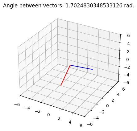

Angle in Radians: 1.722421 rad
Angle in Degrees: 98.69°

--- Equivalency check ---
Algebraic dot product: -3
Geometric dot product: -3.000000
Close enough?          True

Key Takeaways

• Geometric Formula: $\mathbf{a}^{\text{T}}\mathbf{b} = \|\mathbf{a}\|\|\mathbf{b}\|\cos\theta$.
• Angle Solver: Find angles in any dimension using $\theta = \arccos\left(\frac{\mathbf{a}^{\text{T}}\mathbf{b}}{\|\mathbf{a}\|\|\mathbf{b}\|}\right)$.
• Orthogonality: Two vectors are orthogonal if and only if their dot product is zero ($\theta = 90^\circ$).
• Equivalence: The algebraic element-wise sum and geometric cosine projection equations are algebraically identical via the Law of Cosines.
• Cauchy-Schwarz Inequality: $\left|\mathbf{a}^{\text{T}}\mathbf{b}\right| \leq \|\mathbf{a}\|\|\mathbf{b}\|$, with exact equality holding if and only if the vectors are collinear (linearly dependent).