12. Unit Vectors

Unit Vectors

In previous lessons, we saw that the length (magnitude) of a vector is completely independent of its orientation (angle). This means that infinite vectors can point in the exact same direction while having vastly different lengths.

Any set of vectors pointing along the same line are scalar multiples of each other. In many linear algebra, engineering, and machine learning applications, we want to strip away the length of a vector and focus entirely on its direction.

To do this, we scale the vector so that its length is exactly $1$. A vector with a magnitude of $1$ is called a Unit Vector.

1. Formal Definition

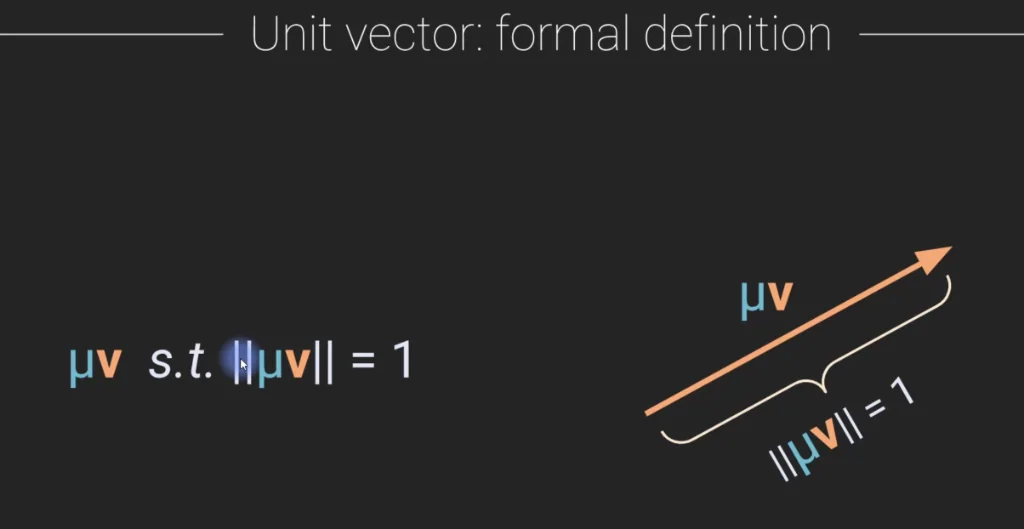
A unit vector is algebraically and geometrically defined as a scaled version of a vector that satisfies a length constraint of one.

Algebraic Definition

If we scale a vector $\mathbf{v}$ by a scalar factor $\mu$, the scaled vector $\mu \mathbf{v}$ is a unit vector if and only if: $$\|\mu \mathbf{v}\| = 1$$

Geometric Definition

Geometrically, scaling any non-zero vector by the correct positive scalar $\mu$ contracts or expands it so that its tip lies exactly on the boundary of a unit circle (in 2D) or unit sphere (in 3D), representing a length of $1$:

2. Normalizing a Vector (How to Choose $\mu$)

To transform an arbitrary vector $\mathbf{v}$ into a unit vector pointing in the same direction, we must select the appropriate scaling factor $\mu$.

The Numerical Analogy

Think about a regular real number, for example, $3$. If you want to scale this number to equal the "unit number" (which is $1$), what scalar must you multiply it by?

You multiply it by its reciprocal: $$\mu \cdot 3 = 1 \quad \implies \quad \mu = \frac{1}{3}$$

The Vector Generalization

We apply the exact same reciprocal concept to vectors. To scale any non-zero vector $\mathbf{v}$ to have a length of $1$, we choose $\mu$ as the reciprocal of the vector's magnitude:

Multiplying the vector $\mathbf{v}$ by this scalar $\mu$ yields the normalized unit vector (often written as $\mathbf{u}$ or with a hat symbol $\mathbf{\hat{v}}$):

3. The Zero Vector Exception

A crucial mathematical exception to unit vectors is the Zero Vector ($\mathbf{0} = [0, 0, \dots, 0]$). The zero vector does not have a corresponding unit vector.

This makes absolute sense both geometrically and algebraically:

• Geometrically: The zero vector is simply a single point located at the origin. It has no length, no magnitude, and thus no defined direction. It is impossible to point in "the same direction" as a point.
• Algebraically: The magnitude of the zero vector is $\|\mathbf{0}\| = 0$. If we attempt to compute the normalization scalar $\mu = \frac{1}{\|\mathbf{0}\|} = \frac{1}{0}$, we encounter a division-by-zero error, which is undefined.
• Numerical Analogy: There is no real number $\mu$ that can multiply $0$ to equal $1$ ($\mu \cdot 0 = 0 \neq 1$).

4. Python Implementation

In NumPy, we normalize a vector by first computing its Euclidian norm using np.linalg.norm() and then dividing the vector by that norm:

import numpy as np
import matplotlib.pyplot as plt

# 1. Define a 2D vector
v1 = np.array([ -3, 6 ])

# 2. Compute the normalization scalar (mu = 1 / norm)
v1_norm = np.linalg.norm(v1)
mu = 1 / v1_norm
v1n = v1 * mu

print(f"Original Vector v1 : {v1}")
print(f"Vector Magnitude    : {v1_norm:.4f}")
print(f"Normalization Scalar: {mu:.4f}")
print(f"Unit Vector v1-norm : {v1n}")
print(f"Normalized Length   : {np.linalg.norm(v1n):.1f}")

# 3. Plot original vector vs normalized vector
plt.figure(figsize=(6, 6))
plt.plot([0, v1[0]], [0, v1[1]], 'b', label='Original Vector v1', linewidth=3)
plt.plot([0, v1n[0]], [0, v1n[1]], 'r', label='Unit Vector v1-norm', linewidth=5)

plt.axis('square')
plt.axis(( -7, 7, -7, 7 ))
plt.grid(True, linestyle='--', alpha=0.6)
plt.legend()
plt.title("Vector Normalization Visualization")
plt.show()

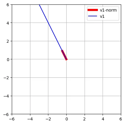
Here is the resulting visualization showing the original vector and its normalized unit equivalent pointing in the exact same direction but scaled to a length of exactly $1$:

Key Takeaways

• Unit Vector: A vector with a magnitude of exactly $1$ ($\|\mathbf{u}\| = 1$), representing direction only.
• Vector Normalization: The process of scaling any non-zero vector $\mathbf{v}$ by $\frac{1}{\|\mathbf{v}\|}$ to create a unit vector in the same direction.
• Zero Vector Boundary: The zero vector has a magnitude of $0$ and no defined direction, meaning it cannot be normalized (division-by-zero is mathematically undefined).