1. Introduction to Vectors

Introduction to Vectors

In linear algebra, one of the most powerful and core concepts is Algebraic-Geometric Dualism. Almost every topic we cover can be expressed and understood in two parallel ways:

• Algebraically: Offering structural precision, sequence manipulation, and ease of high-dimensional scaling.
• Geometrically: Providing spatial intuition, visual interpretability, and physical grounding.

This dualism is extremely powerful because some concepts are much more intuitive in algebraic terms, whereas others are far more interpretable using geometric terms. We begin our journey by exploring both sides of this coin using vectors.

1. The Algebraic Interpretation

Algebraically, a vector is an ordered list of numbers.

Core Properties

• Syntax: Vector elements are typically enclosed by brackets [] (like matrices), angled brackets ⟨⟩, or parentheses ().
• Element Types: The numbers (elements) inside a vector can be integers, fractions, real numbers, complex numbers, rational, or irrational values.
• Order is Meaningful: The sequence of elements is strictly ordered. Changing the sequence changes the vector. For example: $$\begin{bmatrix} 1 \\ 2 \end{bmatrix} \neq \begin{bmatrix} 2 \\ 1 \end{bmatrix}$$
• Dimensionality: The number of elements inside a vector defines its dimensionality.
• $\begin{bmatrix} 1 \\ -2 \end{bmatrix}$ is a $2$-dimensional vector.
• $\begin{bmatrix} 4 \\ -3 \\ 2 \end{bmatrix}$ is a $3$-dimensional vector.
• $\begin{bmatrix} 9 \\ -2.5 \\ 0 \\ 1.2 \\ 7 \end{bmatrix}$ is a $5$-dimensional vector.

Vector Orientations

Vectors can show up in one of two physical orientations:

1. Column Vectors: "Standing up tall and proud," written vertically. This is the standard mathematical convention for vector operations. $$\mathbf{v} = \begin{bmatrix} 1 \\ 2 \end{bmatrix}$$
2. Row Vectors: "Lazy and lying down," written horizontally. In Python and data science, multi-dimensional feature lists are often represented as row vectors. $$\mathbf{u} = \begin{bmatrix} 1 & 2 \end{bmatrix}$$

Notation Conventions

Notations for referencing vectors vary across different courses and textbooks. The most common conventions include:

• Lowercase boldface Latin letters (e.g., $\mathbf{v}$): The standard text-book printing standard.
• Letters with a top arrow (e.g., $\vec{v}$ or $\vec{\mathbf{v}}$): Commonly used when writing notes by hand or when there is ambiguity about whether a letter refers to a vector. Hand-drawn arrows are often represented as half-arrows ($\vec{v}$).

Our Convention: Throughout this course, we will exclusively use lowercase boldface Latin letters (e.g., $\mathbf{v}$, $\mathbf{u}$) to represent vectors. This is crucial because it allows us to easily distinguish them from scalars (written as normal lowercase letters, e.g., $s, x, c$) and matrices (written as uppercase boldface or normal letters, e.g., $\mathbf{A}, \mathbf{M}$).

Algebraic Vector Operations in Python

Let's represent simple 2D and 3D vectors in Python using standard lists and convert or transpose them using NumPy:

import numpy as np
import matplotlib.pyplot as plt

# 2-dimensional vector
v2 = [ 3, -2 ]

# 3-dimensional vector
v3 = [ 4, -3, 2 ]

# Row to column transpose (using NumPy transpose)
v3t = np.transpose(v3)

2. The Geometric Interpretation

Geometrically, a vector is a directed line segment—a straight line possessing both a specific length (magnitude) and a specific direction. The components of the vector specify exactly how far to move along each coordinate axis.

Robustness to Translation (Rigid-body translation)

A vector is only defined by its length and direction. It does not matter where in coordinate space the vector starts. If we draw several parallel arrows of the same length pointing in the same direction in different parts of a grid, they are all geometric representations of the exact same vector!

Visualizing Vectors in 2D

Here is the code to plot our 2D vector $\mathbf{v}_2 = \begin{bmatrix} 3 \\ -2 \end{bmatrix}$ in standard position using Matplotlib:

# Plot the 2D vector
plt.plot([0,v2[0]],[0,v2[1]])
plt.axis('equal')
plt.plot([-4, 4],[0, 0],'k--')
plt.plot([0, 0],[-4, 4],'k--')
plt.grid()
plt.axis((-4, 4, -4, 4))
plt.show()

Ignoring fixed x limits to fulfill fixed data aspect with adjustable data limits.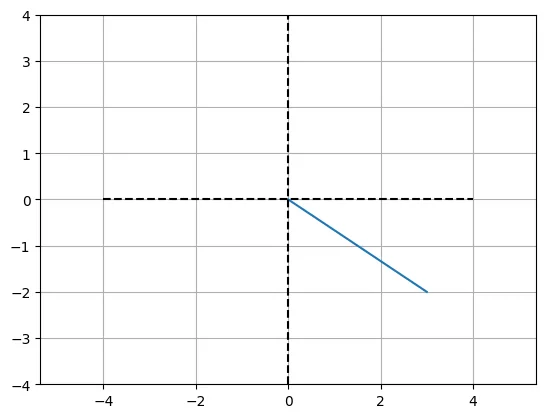

Visualizing Vectors in 3D

Here is the code to plot our 3D vector $\mathbf{v}_3 = \begin{bmatrix} 4 \\ -3 \\ 2 \end{bmatrix}$ using Matplotlib's 3D projection:

# Plot the 3D vector
fig = plt.figure(figsize=plt.figaspect(1))
ax = plt.axes(projection = '3d')
ax.plot([0, v3[0]],[0, v3[1]],[0, v3[2]],linewidth=3)

# Make the plot axes lines look nicer
ax.plot([0, 0],[0, 0],[-4, 4],'k--')
ax.plot([0, 0],[-4, 4],[0, 0],'k--')
ax.plot([-4, 4],[0, 0],[0, 0],'k--')
plt.show()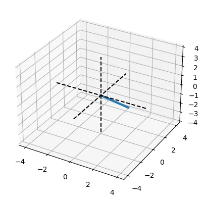

Anatomy of a Vector and Standard Position

• Tail: The starting point of the vector.
• Head: The endpoint, marked by an arrowhead showing the direction.
• Standard Position: When a vector is drawn such that its tail is anchored at the origin $(0, 0, \dots, 0)$, it is said to be in Standard Position. Unless explicitly stated otherwise, we generally assume vectors are in standard position.
• Vector vs. Coordinate Point: A vector is not the same thing as a coordinate point:
• A Coordinate Point refers to a single static dot (location) in space (e.g., the point $(3, -2)$).
• A Vector refers to a displacement or motion (length and direction) that can exist anywhere.
• Note: When a vector is in its standard position, the vector's head directly overlaps with the coordinate point. In this special case, they represent the same coordinates.

3. Vector-Valued Functions

Vectors are not limited to containing only static numbers. They can also contain mathematical functions of a continuous variable! This yields a vector-valued function:

Here, $x$ acts as a continuous parameter. As $x$ varies, the vector sweeps out a coordinate trajectory in $3$-dimensional space. For this specific function, the coordinates trace a beautiful, opening conoid helix (a 3D spiral).