Vector-Scalar Multiplication
Multiplying a vector by a single number is one of the most fundamental operations in linear algebra. Geometrically, it forms the basis of vector scaling, projections, and the concept of linear span. In this lesson, we will explore the standard terminology of linear algebra and dive into the algebraic and geometric interpretations of vector-scalar multiplication.
1. Linear Algebra Terminology
Before we multiply vectors and scalars, let's establish a clear vocabulary. In linear algebra, there are three primary objects we deal with, each with its own strict symbol and naming conventions:
- Matrix: A two-dimensional grid of numbers (rows and columns).
- Notation: Capital boldface Latin letters (e.g., ).
- Vector: A one-dimensional ordered list of numbers.
- Notation: Lowercase boldface Latin letters (e.g., ).
- Scalar: A single, standalone number.
- Notation: Lowercase, non-boldface Greek letters (e.g., ).
| Mathematical Object | Common Name | Standard Notation Symbol | Example Representation |
|---|---|---|---|
| Matrix | Matrix | , , (Capital Boldface Latin) | |
| Vector | Vector | , , (Lowercase Boldface Latin) | |
| Scalar | Scalar | , , (Lowercase Light Greek) | $7$ |
2. The Algebraic Interpretation
Algebraically, multiplying a vector by a scalar means multiplying every individual element of the vector by that scalar.
Numerical Example (3D Vector)
Let's scale the 3D column vector by a scalar :
3. The Geometric Interpretation
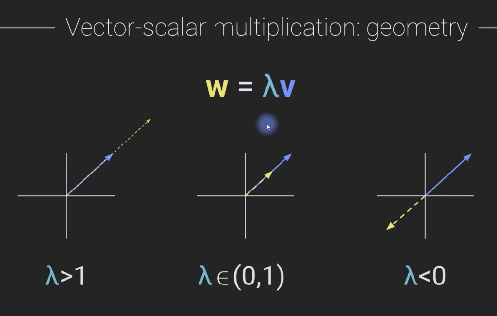
Geometrically, multiplying a vector by a scalar scales (stretches or shrinks) the magnitude of the vector without rotating it off its axis. This scaling effect is exactly why a single number is called a scalar!
Depending on the value of the scalar , we observe three distinct geometric behaviors (excluding and ):
- Stretching (): The scaled vector points in the same direction and grows longer.
- Shrinking (): The scaled vector points in the same direction and grows shorter.
- Direction Reversal (): The scaled vector spins around to point in the exact opposite direction ( rotation) while being stretched or shrunk by the absolute value .
4. The Concept of a 1D Subspace
At first glance, a negative scalar () appears to alter the vector's direction. While true in a colloquial sense, in linear algebra we think of this in terms of subspaces:
💡 Linear Subspaces: The vector and all of its scaled versions () lie on the exact same one-dimensional subspace—an infinitely long straight line passing through the origin.
Because a negative scalar merely slides the vector's head to the opposite half of this infinite line, it has not altered the spatial line (axis) upon which the vector resides. Thus, all scaled versions of a vector share a deep, fundamental relationship.
5. Python Implementation
Here is how to implement vector-scalar multiplication in NumPy and plot the original and scaled vectors in Matplotlib:
import numpy as np
import matplotlib.pyplot as plt

# Define a 2D vector and a scalar multiplier
v1 = np.array([ 3, -1 ])
λ  = 2.3

# Scalar multiplication (vector-scalar modulation)
v1_scaled = v1 * λ

# Plot the vectors
plt.plot([0, v1[0]], [0, v1[1]], 'b', linewidth=3, label='$v_1$')
plt.plot([0, v1_scaled[0]], [0, v1_scaled[1]], 'r:', linewidth=3, label='$\lambda v_1$')

plt.legend()
plt.axis('square')

# Dynamically compute axes boundaries
axlim = max([max(abs(v1)), max(abs(v1_scaled))]) * 1.5
plt.axis((-axlim, axlim, -axlim, axlim))

plt.grid()
plt.show()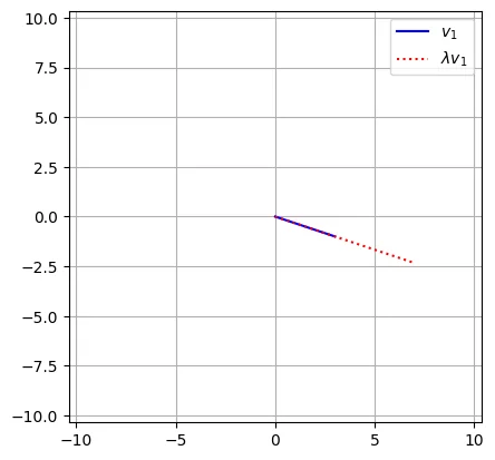
Key Takeaways
- Element-wise Scaling: Algebraically, the scalar scales each component of the vector individually.
- Magnitude Modulation: Geometrically, scalars stretch or shrink a vector's length.
- Negative Scaling: A negative scalar reverses the vector's heading ( flip).
- Subspace Alignment: All scaled variants of a vector are collinear, residing on the same 1D subspace passing through the origin.