10. Cross Product

Vector Cross Product

So far, we have discussed several ways to multiply vectors: the Dot Product (collapsing into a scalar), the Hadamard Product (element-wise vector scaling), and the Outer Product (stretching into a matrix).

In this lesson, we cover a classic vector multiplication method: the Cross Product (written as $\mathbf{v}_1 \times \mathbf{v}_2$). The cross product is a highly specialized operation with deep applications in physics, computer graphics, and 3D coordinate system transformations.

1. Core Rules of the Cross Product

Before diving into the formulas, there are two strict mathematical rules you must memorize:

1. Strict 3D Limitation: The vector cross product is defined if and only if both vectors are three-dimensional ($\mathbb{R}^3$). It is mathematically undefined for 2D vectors, 4D vectors, or any higher-dimensional representations.
2. 3D Output: The resulting product vector is also another 3D vector.

2. The Algebraic Formula (The Crossing Pattern)

The algebraic formula for the cross product appears complex at first glance. However, it is built on a repeating, crossed subtraction pattern.

For two general 3D vectors: $$\mathbf{v}_1 = \begin{bmatrix} x_1 \\ y_1 \\ z_1 \end{bmatrix}, \quad \mathbf{v}_2 = \begin{bmatrix} x_2 \\ y_2 \\ z_2 \end{bmatrix}$$

The cross product is computed as: $$\mathbf{v}_1 \times \mathbf{v}_2 = \begin{bmatrix} y_1 z_2 - z_1 y_2 \\ z_1 x_2 - x_1 z_2 \\ x_1 y_2 - y_1 x_2 \end{bmatrix}$$

Visualizing the Crossing Formula

To see where the terms come from, look at this concrete visual showing a numerical column vector crossed with a symbol vector:

• Row 1 ($x$-component): We ignore the top row of the inputs and cross-multiply the remaining elements: $(2 \cdot c) - (3 \cdot b)$.
• Row 2 ($y$-component): We ignore the middle row of the inputs and cross-multiply: $(3 \cdot a) - (1 \cdot c)$.
• Row 3 ($z$-component): We ignore the bottom row of the inputs and cross-multiply: $(1 \cdot b) - (2 \cdot a)$.

While this formula can be difficult to memorize, computer packages handle this computation effortlessly.

3. Geometric Interpretation (The Normal Vector)

Geometrically, the cross product is incredibly beautiful.

In Euclidean geometry, any two distinct, non-collinear vectors in $\mathbb{R}^3$ define a unique two-dimensional plane.

When you compute the cross product $\mathbf{v}_3 = \mathbf{v}_1 \times \mathbf{v}_2$, the resulting vector $\mathbf{v}_3$ is perfectly orthogonal (perpendicular) to both input vectors, which means it sticks straight out at a $90^\circ$ right angle to the entire spanned plane!

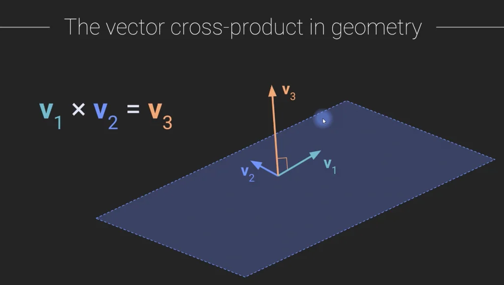
In geometry and computer graphics, this orthogonal vector is called the normal vector to the plane. The normal vector is the primary way we define the orientation of surfaces in 3D space, which is critical for physics engines (torque calculations) and lighting algorithms (ray-tracing).

4. Python Implementation and 3D Visualization

In NumPy, we calculate the cross product using np.cross().

Below is the Python code to compute the cross product both using NumPy and manually, and then render the spanned plane along with the orthogonal normal vector in interactive 3D:

import numpy as np
import matplotlib.pyplot as plt

# 1. Define two 3D vectors
v1  = [ -3,  2, 5 ]
v2  = [  4, -3, 0 ]

# 2. Compute using NumPy's built-in cross product
v3a = np.cross(v1, v2)

# 3. Compute manually using the algebraic cross formula
v3b = [ [v1[1]*v2[2] - v1[2]*v2[1]],
        [v1[2]*v2[0] - v1[0]*v2[2]],
        [v1[0]*v2[1] - v1[1]*v2[0]] ]

print(f"NumPy cross product:  {v3a}")
print(f"Manual cross product:\n{np.array(v3b)}")

# 4. Draw the spanned plane and vectors in 3D
fig = plt.figure(figsize=(8, 8))
ax = plt.axes(projection='3d')

# Generate coordinates for the spanned 2D plane
xx, yy = np.meshgrid(np.linspace(-10, 10, 10), np.linspace(-10, 10, 10))
# Plane equation derived from the normal vector: ax + by + cz = 0 -> z = (-ax - by)/c
zz = (-v3a[0]*xx - v3a[1]*yy) / v3a[2]
ax.plot_surface(xx, yy, zz, alpha=0.15, color='cyan')

# Plot the vectors starting at origin
ax.plot([0, v1[0]], [0, v1[1]], [0, v1[2]], 'k-', linewidth=3, label='Vector v1')
ax.plot([0, v2[0]], [0, v2[1]], [0, v2[2]], 'b-', linewidth=3, label='Vector v2')
ax.plot([0, v3a[0]], [0, v3a[1]], [0, v3a[2]], 'r-', linewidth=3, label='v1 x v2 (Normal Vector)')

# Configure axis and limits
ax.set_xlim([-10, 10])
ax.set_ylim([-10, 10])
ax.set_zlim([-10, 10])
ax.view_init(azim=150, elev=45)
ax.set_title("3D Cross Product: Normal to the Spanned Plane")
ax.legend()
plt.show()

NumPy cross product:  [15 20  1]
Manual cross product:
[[15]
 [20]
 [ 1]]

Here is the high-fidelity 3D visualization generated by the code above:

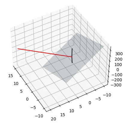
Notice how the red normal vector ($\mathbf{v}_1 \times \mathbf{v}_2$) stands perfectly perpendicular to the cyan-shaded plane defined by the span of $\mathbf{v}_1$ and $\mathbf{v}_2$.

Key Takeaways

• 3D Domain: The cross product $\mathbf{v}_1 \times \mathbf{v}_2$ is defined only for 3D vectors ($n = 3$), resulting in another 3D vector.
• Algebraic Crossing: The components are calculated by ignoring the current row and subtracting crossed products of the remaining elements.
• Geometric Perpendicularity: The product vector is orthogonal (at a $90^\circ$ angle) to the 2D plane spanned by the two input vectors.
• Normal Vector: Used extensively in computer graphics and physics to represent surface orientations and torque.