06-Additional-Matplotlib-Commands-NO_VIDEO

Logarithmic scale

It is also possible to set a logarithmic scale for one or both axes. This functionality is in fact only one application of a more general transformation system in Matplotlib. Each of the axes' scales are set seperately using set_xscale{:python} and set_yscale{:python} methods which accept one parameter (with the value "log" in this case):

python

fig, axes = plt.subplots(1, 2, figsize=(10,4))
      
axes[0].plot(x, x**2, x, np.exp(x))
axes[0].set_title("Normal scale")

axes[1].plot(x, x**2, x, np.exp(x))
axes[1].set_yscale("log")
axes[1].set_title("Logarithmic scale (y)");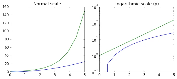

Placement of ticks and custom tick labels

We can explicitly determine where we want the axis ticks with set_xticks{:python} and set_yticks{:python}, which both take a list of values for where on the axis the ticks are to be placed. We can also use the set_xticklabels{:python} and set_yticklabels{:python} methods to provide a list of custom text labels for each tick location:

python

fig, ax = plt.subplots(figsize=(10, 4))

ax.plot(x, x**2, x, x**3, lw=2)

ax.set_xticks([1, 2, 3, 4, 5])
ax.set_xticklabels([r'$\alpha$', r'$\beta$', r'$\gamma$', r'$\delta$', r'$\epsilon$'], fontsize=18)

yticks = [0, 50, 100, 150]
ax.set_yticks(yticks)
ax.set_yticklabels(["$%.1f$" % y for y in yticks], fontsize=18); # use LaTeX formatted labels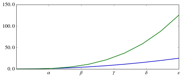

There are a number of more advanced methods for controlling major and minor tick placement in matplotlib figures, such as automatic placement according to different policies. See http://matplotlib.org/api/ticker_api.html for details.

Scientific notation

With large numbers on axes, it is often better use scientific notation:

python

fig, ax = plt.subplots(1, 1)
      
ax.plot(x, x**2, x, np.exp(x))
ax.set_title("scientific notation")

ax.set_yticks([0, 50, 100, 150])

from matplotlib import ticker
formatter = ticker.ScalarFormatter(useMathText=True)
formatter.set_scientific(True) 
formatter.set_powerlimits((-1,1)) 
ax.yaxis.set_major_formatter(formatter)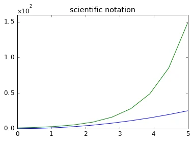

Axis number and axis label spacing

python

# distance between x and y axis and the numbers on the axes
matplotlib.rcParams['xtick.major.pad'] = 5
matplotlib.rcParams['ytick.major.pad'] = 5

fig, ax = plt.subplots(1, 1)
      
ax.plot(x, x**2, x, np.exp(x))
ax.set_yticks([0, 50, 100, 150])

ax.set_title("label and axis spacing")

# padding between axis label and axis numbers
ax.xaxis.labelpad = 5
ax.yaxis.labelpad = 5

ax.set_xlabel("x")
ax.set_ylabel("y");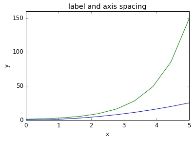

python

# restore defaults
matplotlib.rcParams['xtick.major.pad'] = 3
matplotlib.rcParams['ytick.major.pad'] = 3

Axis position adjustments

Unfortunately, when saving figures the labels are sometimes clipped, and it can be necessary to adjust the positions of axes a little bit. This can be done using subplots_adjust{:python}:

python

fig, ax = plt.subplots(1, 1)
      
ax.plot(x, x**2, x, np.exp(x))
ax.set_yticks([0, 50, 100, 150])

ax.set_title("title")
ax.set_xlabel("x")
ax.set_ylabel("y")

fig.subplots_adjust(left=0.15, right=.9, bottom=0.1, top=0.9);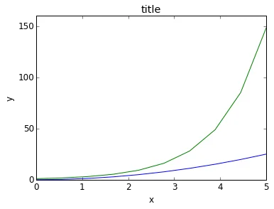

Axis grid

With the grid{:python} method in the axis object, we can turn on and off grid lines. We can also customize the appearance of the grid lines using the same keyword arguments as the plot{:python} function:

python

fig, axes = plt.subplots(1, 2, figsize=(10,3))

# default grid appearance
axes[0].plot(x, x**2, x, x**3, lw=2)
axes[0].grid(True)

# custom grid appearance
axes[1].plot(x, x**2, x, x**3, lw=2)
axes[1].grid(color='b', alpha=0.5, linestyle='dashed', linewidth=0.5)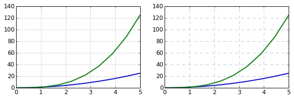

Axis spines

We can also change the properties of axis spines:

python

fig, ax = plt.subplots(figsize=(6,2))

ax.spines['bottom'].set_color('blue')
ax.spines['top'].set_color('blue')

ax.spines['left'].set_color('red')
ax.spines['left'].set_linewidth(2)

# turn off axis spine to the right
ax.spines['right'].set_color("none")
ax.yaxis.tick_left() # only ticks on the left side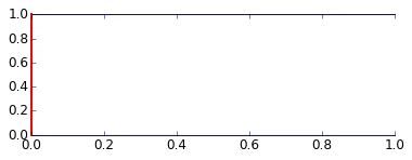

Twin axes

Sometimes it is useful to have dual x or y axes in a figure; for example, when plotting curves with different units together. Matplotlib supports this with the twinx{:python} and twiny{:python} functions:

python

fig, ax1 = plt.subplots()

ax1.plot(x, x**2, lw=2, color="blue")
ax1.set_ylabel(r"area $(m^2)$", fontsize=18, color="blue")
for label in ax1.get_yticklabels():
    label.set_color("blue")
    
ax2 = ax1.twinx()
ax2.plot(x, x**3, lw=2, color="red")
ax2.set_ylabel(r"volume $(m^3)$", fontsize=18, color="red")
for label in ax2.get_yticklabels():
    label.set_color("red")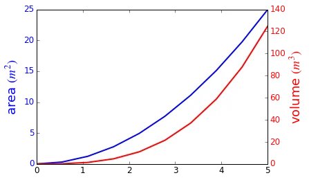

Axes where x and y is zero

python

fig, ax = plt.subplots()

ax.spines['right'].set_color('none')
ax.spines['top'].set_color('none')

ax.xaxis.set_ticks_position('bottom')
ax.spines['bottom'].set_position(('data',0)) # set position of x spine to x=0

ax.yaxis.set_ticks_position('left')
ax.spines['left'].set_position(('data',0))   # set position of y spine to y=0

xx = np.linspace(-0.75, 1., 100)
ax.plot(xx, xx**3);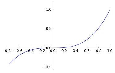

Other 2D plot styles

In addition to the regular plot{:python} method, there are a number of other functions for generating different kind of plots. See the matplotlib plot gallery for a complete list of available plot types: http://matplotlib.org/gallery.html. Some of the more useful ones are show below:

python

n = np.array([0,1,2,3,4,5])

python

fig, axes = plt.subplots(1, 4, figsize=(12,3))

axes[0].scatter(xx, xx + 0.25*np.random.randn(len(xx)))
axes[0].set_title("scatter")

axes[1].step(n, n**2, lw=2)
axes[1].set_title("step")

axes[2].bar(n, n**2, align="center", width=0.5, alpha=0.5)
axes[2].set_title("bar")

axes[3].fill_between(x, x**2, x**3, color="green", alpha=0.5);
axes[3].set_title("fill_between");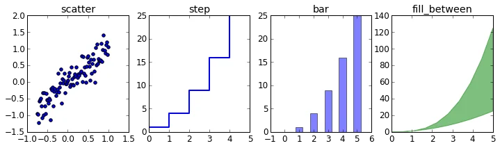

Text annotation

Annotating text in matplotlib figures can be done using the text{:python} function. It supports LaTeX formatting just like axis label texts and titles:

python

fig, ax = plt.subplots()

ax.plot(xx, xx**2, xx, xx**3)

ax.text(0.15, 0.2, r"$y=x^2$", fontsize=20, color="blue")
ax.text(0.65, 0.1, r"$y=x^3$", fontsize=20, color="green");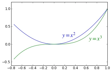

Figures with multiple subplots and insets

Axes can be added to a matplotlib Figure canvas manually using fig.add_axes{:python} or using a sub-figure layout manager such as subplots{:python}, subplot2grid{:python}, or gridspec{:python}:

subplots

python

fig, ax = plt.subplots(2, 3)
fig.tight_layout()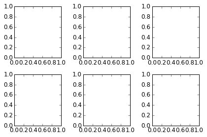

subplot2grid

python

fig = plt.figure()
ax1 = plt.subplot2grid((3,3), (0,0), colspan=3)
ax2 = plt.subplot2grid((3,3), (1,0), colspan=2)
ax3 = plt.subplot2grid((3,3), (1,2), rowspan=2)
ax4 = plt.subplot2grid((3,3), (2,0))
ax5 = plt.subplot2grid((3,3), (2,1))
fig.tight_layout()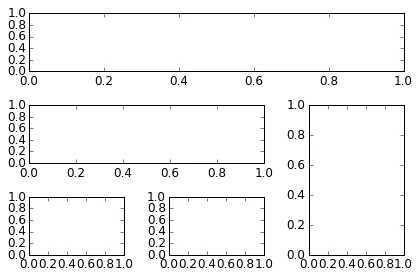

gridspec

python

fig = plt.figure()

gs = gridspec.GridSpec(2, 3, height_ratios=[2,1], width_ratios=[1,2,1])
for g in gs:
    ax = fig.add_subplot(g)
    
fig.tight_layout()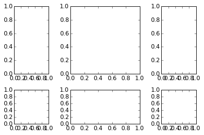

add_axes

Manually adding axes with add_axes{:python} is useful for adding insets to figures:

python

fig, ax = plt.subplots()

ax.plot(xx, xx**2, xx, xx**3)
fig.tight_layout()

# inset
inset_ax = fig.add_axes([0.2, 0.55, 0.35, 0.35]) # X, Y, width, height

inset_ax.plot(xx, xx**2, xx, xx**3)
inset_ax.set_title('zoom near origin')

# set axis range
inset_ax.set_xlim(-.2, .2)
inset_ax.set_ylim(-.005, .01)

# set axis tick locations
inset_ax.set_yticks([0, 0.005, 0.01])
inset_ax.set_xticks([-0.1,0,.1]);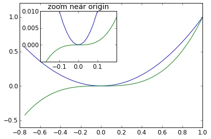

Colormap and contour figures

Colormaps and contour figures are useful for plotting functions of two variables. In most of these functions we will use a colormap to encode one dimension of the data. There are a number of predefined colormaps. It is relatively straightforward to define custom colormaps. For a list of pre-defined colormaps, see: http://www.scipy.org/Cookbook/Matplotlib/Show_colormaps

python

alpha = 0.7
phi_ext = 2 * np.pi * 0.5

def flux_qubit_potential(phi_m, phi_p):
    return 2 + alpha - 2 * np.cos(phi_p) * np.cos(phi_m) - alpha * np.cos(phi_ext - 2*phi_p)

python

phi_m = np.linspace(0, 2*np.pi, 100)
phi_p = np.linspace(0, 2*np.pi, 100)
X,Y = np.meshgrid(phi_p, phi_m)
Z = flux_qubit_potential(X, Y).T

pcolor

python

fig, ax = plt.subplots()

p = ax.pcolor(X/(2*np.pi), Y/(2*np.pi), Z, cmap=matplotlib.cm.RdBu, vmin=abs(Z).min(), vmax=abs(Z).max())
cb = fig.colorbar(p, ax=ax)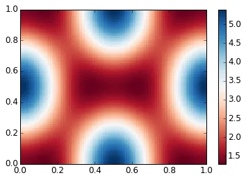

imshow

python

fig, ax = plt.subplots()

im = ax.imshow(Z, cmap=matplotlib.cm.RdBu, vmin=abs(Z).min(), vmax=abs(Z).max(), extent=[0, 1, 0, 1])
im.set_interpolation('bilinear')

cb = fig.colorbar(im, ax=ax)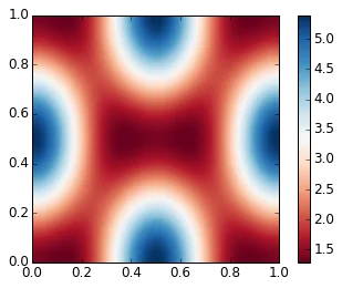

contour

python

fig, ax = plt.subplots()

cnt = ax.contour(Z, cmap=matplotlib.cm.RdBu, vmin=abs(Z).min(), vmax=abs(Z).max(), extent=[0, 1, 0, 1])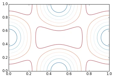

3D figures

To use 3D graphics in matplotlib, we first need to create an instance of the Axes3D{:python} class. 3D axes can be added to a matplotlib figure canvas in exactly the same way as 2D axes; or, more conveniently, by passing a projection='3d'{:python} keyword argument to the add_axes{:python} or add_subplot{:python} methods.

python

from mpl_toolkits.mplot3d.axes3d import Axes3D

Surface plots

python

fig = plt.figure(figsize=(14,6))

# `ax` is a 3D-aware axis instance because of the projection='3d' keyword argument to add_subplot
ax = fig.add_subplot(1, 2, 1, projection='3d')

p = ax.plot_surface(X, Y, Z, rstride=4, cstride=4, linewidth=0)

# surface_plot with color grading and color bar
ax = fig.add_subplot(1, 2, 2, projection='3d')
p = ax.plot_surface(X, Y, Z, rstride=1, cstride=1, cmap=matplotlib.cm.coolwarm, linewidth=0, antialiased=False)
cb = fig.colorbar(p, shrink=0.5)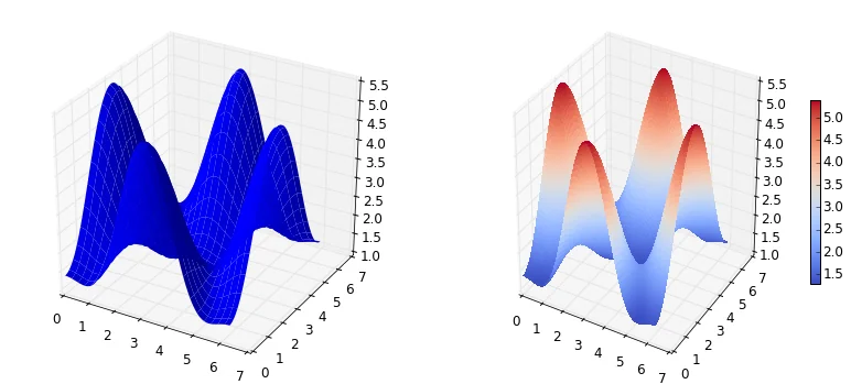

Wire-frame plot

python

fig = plt.figure(figsize=(8,6))

ax = fig.add_subplot(1, 1, 1, projection='3d')

p = ax.plot_wireframe(X, Y, Z, rstride=4, cstride=4)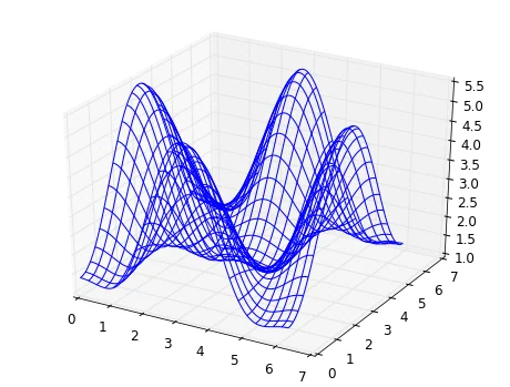

Coutour plots with projections

python

fig = plt.figure(figsize=(8,6))

ax = fig.add_subplot(1,1,1, projection='3d')

ax.plot_surface(X, Y, Z, rstride=4, cstride=4, alpha=0.25)
cset = ax.contour(X, Y, Z, zdir='z', offset=-np.pi, cmap=matplotlib.cm.coolwarm)
cset = ax.contour(X, Y, Z, zdir='x', offset=-np.pi, cmap=matplotlib.cm.coolwarm)
cset = ax.contour(X, Y, Z, zdir='y', offset=3*np.pi, cmap=matplotlib.cm.coolwarm)

ax.set_xlim3d(-np.pi, 2*np.pi);
ax.set_ylim3d(0, 3*np.pi);
ax.set_zlim3d(-np.pi, 2*np.pi);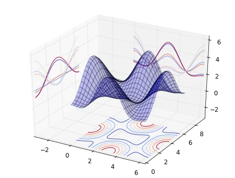

06-Additional-Matplotlib-Commands-NO_VIDEO

Logarithmic scale

Placement of ticks and custom tick labels

Scientific notation

Axis number and axis label spacing

Axis position adjustments

Axis grid

Axis spines

Twin axes

Axes where x and y is zero

Other 2D plot styles

Text annotation

Figures with multiple subplots and insets

subplots

subplot2grid

gridspec

add_axes

Colormap and contour figures

pcolor

imshow

contour

3D figures

Surface plots

Wire-frame plot

Coutour plots with projections

Further reading