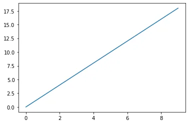
00-Matplotlib-Basics | Driptanil Datta

Introduction

Matplotlib is the "grandfather" library of data visualization with Python. It was created by John Hunter. He created it to try to replicate MatLab's (another programming language) plotting capabilities in Python. So if you happen to be familiar with matlab, matplotlib will feel natural to you.

It is an excellent 2D and 3D graphics library for generating scientific figures.

Some of the major Pros of Matplotlib are:

Generally easy to get started for simple plots
Support for custom labels and texts
Great control of every element in a figure
High-quality output in many formats
Very customizable in general

Matplotlib allows you to create reproducible figures programmatically. Let's learn how to use it! Before continuing this lecture, I encourage you just to explore the official Matplotlib web page: http://matplotlib.org/

Installation

If you are using our environment, its already installed for you. If you are not using our environment (not recommended), you'll need to install matplotlib first with either:

conda install matplotlib or

pip install matplotlib

Importing

Import the matplotlib.pyplot{:python} module under the name plt{:python} (the tidy way):

python

# COMMON MISTAKE!
# DON'T FORGET THE .PYPLOT part

import matplotlib.pyplot as plt

NOTE: If you are using an older version of jupyter, you need to run a "magic" command to see the plots inline with the notebook. Users of jupyter notebook 1.0 and above, don't need to run the cell below:

python

%matplotlib inline

*NOTE: For users running .py scripts in an IDE like PyCharm or Sublime Text Editor. You will not see the plots in a notebook, instead if you are using another editor, you'll use: plt.show() at the end of all your plotting commands to have the figure pop up in another window.*

Basic Example

Let's walk through a very simple example using two numpy arrays:

Basic Array Plot

Let's walk through a very simple example using two numpy arrays. You can also use lists, but most likely you'll be passing numpy arrays or pandas columns (which essentially also behave like arrays).

The data we want to plot:

python

x = np.arange(0,10)

python

y = 2*x

python

Out · result

array([0, 1, 2, 3, 4, 5, 6, 7, 8, 9])

python

Out · result

array([ 0,  2,  4,  6,  8, 10, 12, 14, 16, 18])

Using Matplotlib with plt.plot() function calls

Basic Matplotlib Commands

We can create a very simple line plot using the following ( I encourage you to pause and use Shift+Tab along the way to check out the document strings for the functions we are using).

python

plt.plot(x, y) 
plt.xlabel('X Axis Title Here')
plt.ylabel('Y Axis Title Here')
plt.title('String Title Here')
plt.show() # Required for non-jupyter users , but also removes Out[] info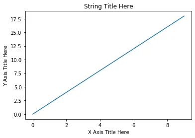

Editing more figure parameters

python

plt.plot(x, y) 
plt.xlabel('X Axis Title Here')
plt.ylabel('Y Axis Title Here')
plt.title('String Title Here')
plt.xlim(0,6) # Lower Limit, Upper Limit
plt.ylim(0,12) # Lower Limit, Upper Limit
plt.show() # Required for non-jupyter users , but also removes Out[] info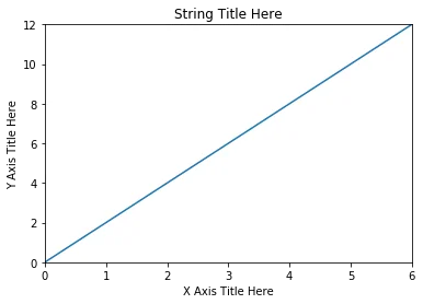

Exporting a plot

python

help(plt.savefig)

Out · stdout

Help on function savefig in module matplotlib.pyplot:

savefig(*args, **kwargs)
    Save the current figure.

106 more lines

    Call signature::
    
      savefig(fname, dpi=None, facecolor='w', edgecolor='w',
              orientation='portrait', papertype=None, format=None,
              transparent=False, bbox_inches=None, pad_inches=0.1,
              frameon=None, metadata=None)
    
    The output formats available depend on the backend being used.
    
    Parameters
    ----------
    
    fname : str or PathLike or file-like object
        A path, or a Python file-like object, or
        possibly some backend-dependent object such as
        `matplotlib.backends.backend_pdf.PdfPages`.
    
        If *format* is not set, then the output format is inferred from
        the extension of *fname*, if any, and from :rc:`savefig.format`
        otherwise.  If *format* is set, it determines the output format.
    
        Hence, if *fname* is not a path or has no extension, remember to
        specify *format* to ensure that the correct backend is used.
    
    Other Parameters
    ----------------
    
    dpi : [ *None* | scalar > 0 | 'figure' ]
        The resolution in dots per inch.  If *None*, defaults to
        :rc:`savefig.dpi`.  If 'figure', uses the figure's dpi value.
    
    quality : [ *None* | 1 <= scalar <= 100 ]
        The image quality, on a scale from 1 (worst) to 95 (best).
        Applicable only if *format* is jpg or jpeg, ignored otherwise.
        If *None*, defaults to :rc:`savefig.jpeg_quality` (95 by default).
        Values above 95 should be avoided; 100 completely disables the
        JPEG quantization stage.
    
    optimize : bool
        If *True*, indicates that the JPEG encoder should make an extra
        pass over the image in order to select optimal encoder settings.
        Applicable only if *format* is jpg or jpeg, ignored otherwise.
        Is *False* by default.
    
    progressive : bool
        If *True*, indicates that this image should be stored as a
        progressive JPEG file. Applicable only if *format* is jpg or
        jpeg, ignored otherwise. Is *False* by default.
    
    facecolor : color spec or None, optional
        The facecolor of the figure; if *None*, defaults to
        :rc:`savefig.facecolor`.
    
    edgecolor : color spec or None, optional
        The edgecolor of the figure; if *None*, defaults to
        :rc:`savefig.edgecolor`
    
    orientation : {'landscape', 'portrait'}
        Currently only supported by the postscript backend.
    
    papertype : str
        One of 'letter', 'legal', 'executive', 'ledger', 'a0' through
        'a10', 'b0' through 'b10'. Only supported for postscript
        output.
    
    format : str
        The file format, e.g. 'png', 'pdf', 'svg', ... The behavior when
        this is unset is documented under *fname*.
    
    transparent : bool
        If *True*, the axes patches will all be transparent; the
        figure patch will also be transparent unless facecolor
        and/or edgecolor are specified via kwargs.
        This is useful, for example, for displaying
        a plot on top of a colored background on a web page.  The
        transparency of these patches will be restored to their
        original values upon exit of this function.
    
    bbox_inches : str or `~matplotlib.transforms.Bbox`, optional
        Bbox in inches. Only the given portion of the figure is
        saved. If 'tight', try to figure out the tight bbox of
        the figure. If None, use savefig.bbox
    
    pad_inches : scalar, optional
        Amount of padding around the figure when bbox_inches is
        'tight'. If None, use savefig.pad_inches
    
    bbox_extra_artists : list of `~matplotlib.artist.Artist`, optional
        A list of extra artists that will be considered when the
        tight bbox is calculated.
    
    metadata : dict, optional
        Key/value pairs to store in the image metadata. The supported keys
        and defaults depend on the image format and backend:
    
        - 'png' with Agg backend: See the parameter ``metadata`` of
          `~.FigureCanvasAgg.print_png`.
        - 'pdf' with pdf backend: See the parameter ``metadata`` of
          `~.backend_pdf.PdfPages`.
        - 'eps' and 'ps' with PS backend: Only 'Creator' is supported.
    
    pil_kwargs : dict, optional
        Additional keyword arguments that are passed to `PIL.Image.save`
        when saving the figure.  Only applicable for formats that are saved
        using Pillow, i.e. JPEG, TIFF, and (if the keyword is set to a
        non-None value) PNG.

python

plt.plot(x,y)
plt.savefig('example.png')