m = np.linspace(0,10,11)

print(f"The array m should look like this: \n\n{m}")The array m should look like this:
[ 0. 1. 2. 3. 4. 5. 6. 7. 8. 9. 10.]c = 3 * 10**8 # Speed of LightE = mc*2print(f"The array E should look like this: \n\n {E}")The array E should look like this:
[0.0e+00 9.0e+16 1.8e+17 2.7e+17 3.6e+17 4.5e+17 5.4e+17 6.3e+17 7.2e+17
8.1e+17 9.0e+17]Part Two: Plotting E=mc^2
Now that we have the arrays E and m, we can plot this to see the relationship between Energy and Mass.
TASK: Import what you need from Matplotlib to plot out graphs:
TASK: Recreate the plot shown below which maps out E=mc^2 using the arrays we created in the previous task. Note the labels, titles, color, and axis limits. You don't need to match perfectly, but you should attempt to re-create each major component.
# CODE HERE# DON"T RUN THE CELL BELOW< THAT WILL ERASE THE PLOT!plt.plot(m,E,color='red',lw=5)
plt.title("E=mc^2")
plt.xlabel("Mass in Grams")
plt.ylabel("Energy in Joules")
plt.xlim(0,10)
plt.show()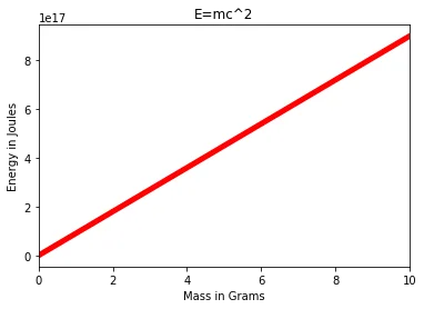
Part Three (BONUS)
Can you figure out how to plot this on a logarthimic scale on the y axis? Place a grid along the y axis ticks as well. We didn't show this in the videos, but you should be able to figure this out by referencing Google, StackOverflow, Matplotlib Docs, or even our "Additional Matplotlib Commands" notebook. The plot we show here only required two more lines of code for the changes.
# CODE HERE# DONT RUN THE CELL BELOW! THAT WILL ERASE THE PLOT!plt.plot(m,E,color='red',lw=5)
plt.title("E=mc^2")
plt.xlabel("Mass in Grams")
plt.ylabel("Energy in Joules")
plt.xlim(0,10)
# LOG SCALE
plt.yscale("log")
plt.grid(which='both',axis='y')
plt.show()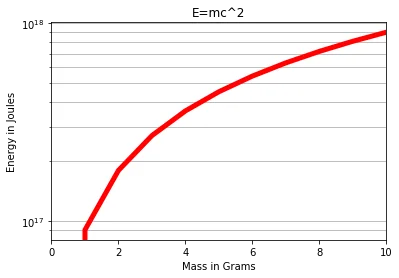
Task Two: Creating plots from data points
In finance, the yield curve is a curve showing several yields to maturity or interest rates across different contract lengths (2 month, 2 year, 20 year, etc. ...) for a similar debt contract. The curve shows the relation between the (level of the) interest rate (or cost of borrowing) and the time to maturity, known as the "term", of the debt for a given borrower in a given currency.
The U.S. dollar interest rates paid on U.S. Treasury securities for various maturities are closely watched by many traders, and are commonly plotted on a graph such as the one on the right, which is informally called "the yield curve".
For this exercise, we will give you the data for the yield curves at two separate points in time. Then we will ask you to create some plots from this data.
Part One: Yield Curve Data
We've obtained some yeild curve data for you from the US Treasury Dept.. The data shows the interest paid for a US Treasury bond for a certain contract length. The labels list shows the corresponding contract length per index position.
TASK: Run the cell below to create the lists for plotting.
labels = ['1 Mo','3 Mo','6 Mo','1 Yr','2 Yr','3 Yr','5 Yr','7 Yr','10 Yr','20 Yr','30 Yr']

july16_2007 =[4.75,4.98,5.08,5.01,4.89,4.89,4.95,4.99,5.05,5.21,5.14]
july16_2020 = [0.12,0.11,0.13,0.14,0.16,0.17,0.28,0.46,0.62,1.09,1.31]
TASK: Figure out how to plot both curves on the same Figure. Add a legend to show which curve corresponds to a certain year.
# CODE HERE# DONT RUN THE CELL BELOW! IT WILL ERASE THE PLOT!# Create Figure (empty canvas)
fig = plt.figure()
# Add set of axes to figure
axes = fig.add_axes([0, 0, 1, 1]) # left, bottom, width, height (range 0 to 1)
# Plot on that set of axes
axes.plot(labels, july16_2007,label='july16_2007')
axes.plot(labels,july16_2020,label='july16_2020')
plt.legend()
plt.show()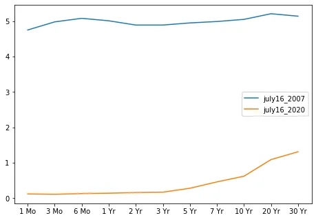
*TASK: The legend in the plot above looks a little strange in the middle of the curves. While it is not blocking anything, it would be nicer if it were outside the plot. Figure out how to move the legend outside the main Figure plot.*
# CODE HERE# DONT RUN THE CELL BELOW! IT WILL ERASE THE PLOT!# Create Figure (empty canvas)
fig = plt.figure()
# Add set of axes to figure
axes = fig.add_axes([0, 0, 1, 1]) # left, bottom, width, height (range 0 to 1)
# Plot on that set of axes
axes.plot(labels, july16_2007,label='july16_2007')
axes.plot(labels,july16_2020,label='july16_2020')
plt.legend(loc=(1.04,0.5))
plt.show()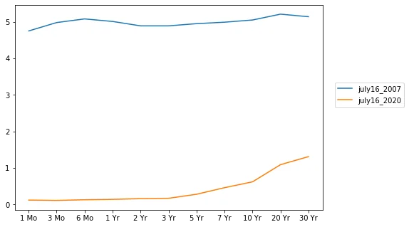
TASK: While the plot above clearly shows how rates fell from 2007 to 2020, putting these on the same plot makes it difficult to discern the rate differences within the same year. Use .suplots() to create the plot figure below, which shows each year's yield curve.
# CODE HERE# DONT RUN THE CELL BELOW! IT WILL ERASE THE PLOT!fig,axes = plt.subplots(nrows=2,ncols=1,figsize=(12,8))
axes[0].plot(labels, july16_2007,label='july16_2007')
axes[0].set_title("July 16th, 2007")
axes[1].plot(labels,july16_2020,label='july16_2020')
axes[1].set_title("July 16th, 2020")
plt.show()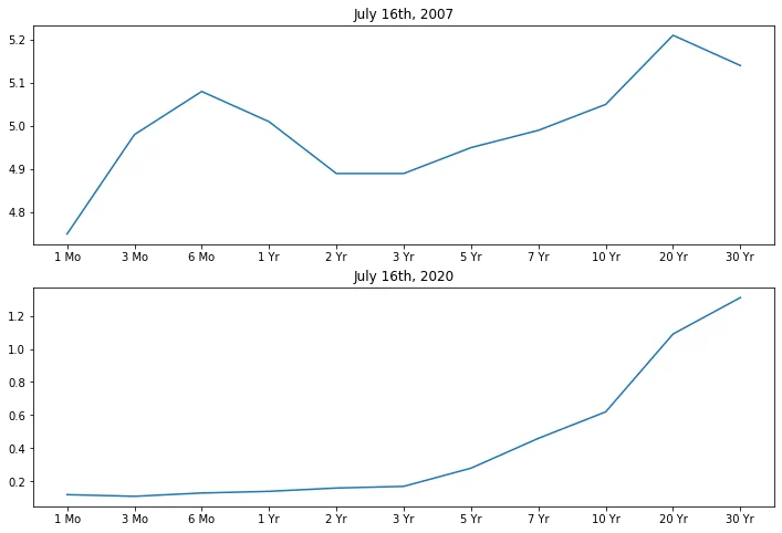
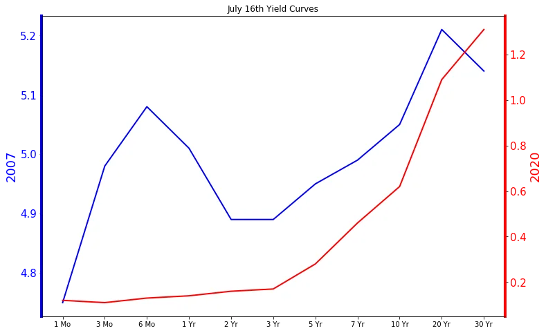
BONUS CHALLENGE TASK: Try to recreate the plot below that uses twin axes. While this plot may actually be more confusing than helpful, its a good exercise in Matplotlib control.
# CODE HERE# DONT RUN THE CELL BELOW! IT ERASES THE PLOT!fig, ax1 = plt.subplots(figsize=(12,8))
ax1.plot(labels,july16_2007, lw=2, color="blue")
ax1.set_ylabel("2007", fontsize=18, color="blue")
ax1.spines['left'].set_color('blue')
ax1.spines['left'].set_linewidth(4)
for label in ax1.get_yticklabels():
label.set_color("blue")
plt.yticks(fontsize=15)
ax2 = ax1.twinx()
ax2.plot(labels,july16_2020, lw=2, color="red")
ax2.set_ylabel("2020", fontsize=18, color="red")
ax2.spines['right'].set_color('red')
ax2.spines['right'].set_linewidth(4)
for label in ax2.get_yticklabels():
label.set_color("red")
ax1.set_title("July 16th Yield Curves");
plt.yticks(fontsize=15)(array([0. , 0.2, 0.4, 0.6, 0.8, 1. , 1.2, 1.4]),
<a list of 8 Text yticklabel objects>)