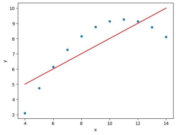
df = pd.read_csv("Advertising.csv")df.head()TV
radio
newspaper
sales
024 more lines
230.1
37.8
69.2
22.1
1
44.5
39.3
45.1
10.4
2
17.2
45.9
69.3
9.3
3
151.5
41.3
58.5
18.5
4
180.8
10.8
58.4
12.9fig,axes = plt.subplots(nrows=1, ncols=3, figsize=(16,6))
axes[0].plot(df['TV'], df['sales'], 'o')
axes[0].set_ylabel('Sales')
axes[0].set_xlabel('TV Advertising Budget')
axes[1].plot(df['radio'], df['sales'], 'o')
axes[1].set_ylabel('Sales')
axes[1].set_xlabel('Radio Advertising Budget')
axes[2].plot(df['newspaper'], df['sales'], 'o')
axes[2].set_ylabel('Sales')
axes[2].set_xlabel('Newspaper Advertising Budget')Text(0.5, 0, 'Newspaper Advertising Budget')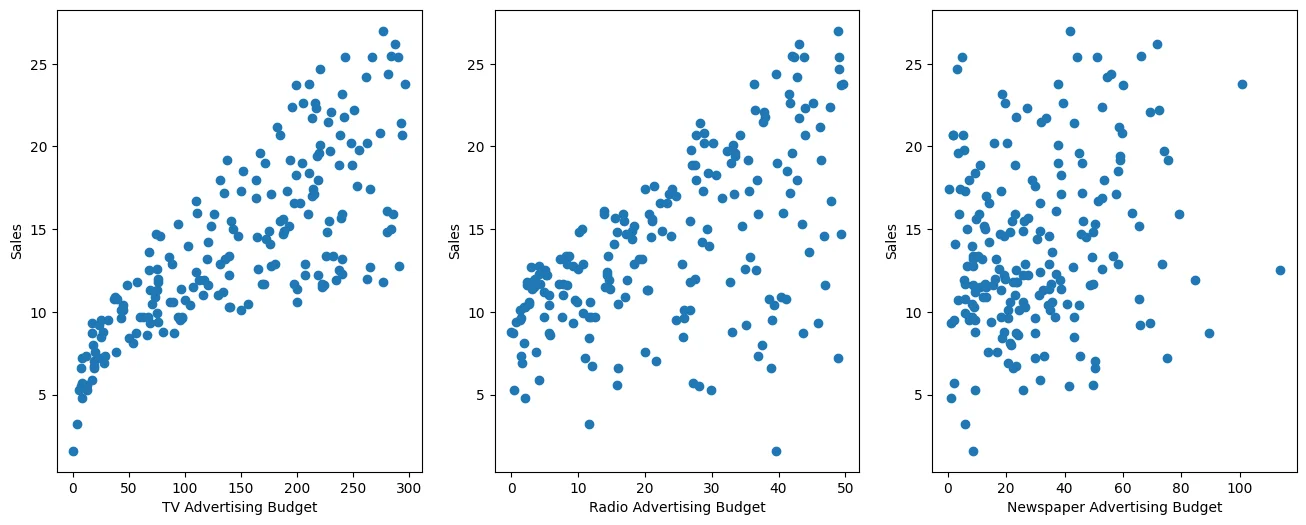
sns.pairplot(df, diag_kind='kde')<seaborn.axisgrid.PairGrid at 0x121816960>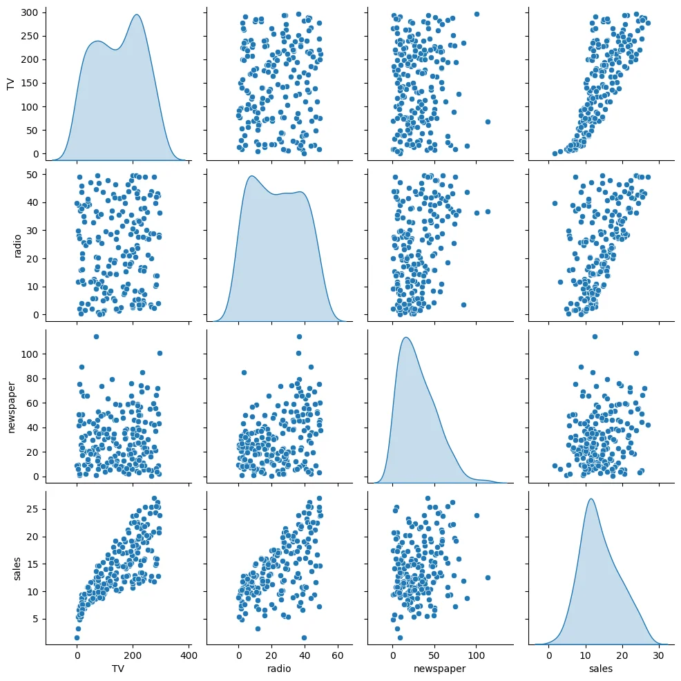
X = df.drop('sales', axis=1)
y = df['sales']from sklearn.model_selection import train_test_split
X_train, X_test, y_train, y_test = train_test_split(X, y, test_size=0.2, random_state=42)X_trainTV
radio
newspaper
79
116.043 more lines
7.7
23.1
197
177.0
9.3
6.4
38
43.1
26.7
35.1
24
62.3
12.6
18.3
122
224.0
2.4
15.6
...
...
...
...
106
25.0
11.0
29.7
14
204.1
32.9
46.0
92
217.7
33.5
59.0
179
165.6
10.0
17.6
102
280.2
10.1
21.4
160 rows × 3 columnsy_train79 11.0
197 12.8
38 10.1
24 9.7
122 11.67 more lines
       ...
106     7.2
14     19.0
92     19.4
179    12.6
102    14.8
Name: sales, Length: 160, dtype: float64from sklearn.linear_model import LinearRegressionmodel = LinearRegression()
# Model Training on Data
model.fit(X_train, y_train)LinearRegression()In a Jupyter environment, please rerun this cell to show the HTML representation or trust the notebook.
On GitHub, the HTML representation is unable to render, please try loading this page with nbviewer.org.
LinearRegression
?Documentation for LinearRegressioniFitted
Parameters10 more lines
fit_intercept
True
copy_X
True
tol
1e-06
n_jobs
None
positive
Falsetest_predictions = model.predict(X_test)test_predictionsarray([16.4080242 , 20.88988209, 21.55384318, 10.60850256, 22.11237326,
13.10559172, 21.05719192, 7.46101034, 13.60634581, 15.15506967,
9.04831992, 6.65328312, 14.34554487, 8.90349333, 9.68959028,
12.16494386, 8.73628397, 16.26507258, 10.27759582, 18.83109103,
19.56036653, 13.25103464, 12.33620695, 21.30695132, 7.82740305,3 more lines
        5.80957448, 20.75753231, 11.98138077,  9.18349576,  8.5066991 ,
       12.46646769, 10.00337695, 21.3876709 , 12.24966368, 18.26661538,
20.13766267, 14.05514005, 20.85411186, 11.0174441 , 4.56899622])from sklearn.metrics import mean_absolute_error,mean_squared_errorMAE = mean_absolute_error(y_test, test_predictions)
MSE = mean_squared_error(y_test, test_predictions)
RMSE = np.sqrt(MSE)print(f"Mean Absolute Error: {MAE}")
print(f"Mean Squared Error: {MSE}")
print(f"Root Mean Squared Error: {RMSE}")Mean Absolute Error: 1.4607567168117606
Mean Squared Error: 3.174097353976105
Root Mean Squared Error: 1.7815996615334504df['sales'].mean()np.float64(14.0225)quartet = pd.read_csv('anscombes_quartet1.csv')quartet['pred_y'] = 3 + 0.5 * quartet['x']
quartet['residual'] = quartet['y'] - quartet['pred_y']
sns.scatterplot(data=quartet, x='x', y='y')
sns.lineplot(data=quartet, x='x', y='pred_y', color='red')
plt.vlines(x=quartet['x'], ymin=quartet['pred_y'], ymax=quartet['y'], color='green', alpha=0.5)<matplotlib.collections.LineCollection at 0x1245f70b0>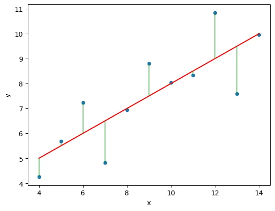
sns.kdeplot(quartet['residual'])<Axes: xlabel='residual', ylabel='Density'>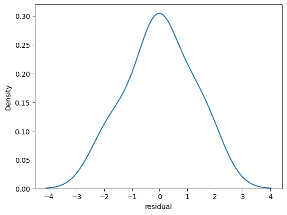
sns.scatterplot(data=quartet,x='y',y='residual')
plt.axhline(y=0, color='r', linestyle='--')<matplotlib.lines.Line2D at 0x124730d40>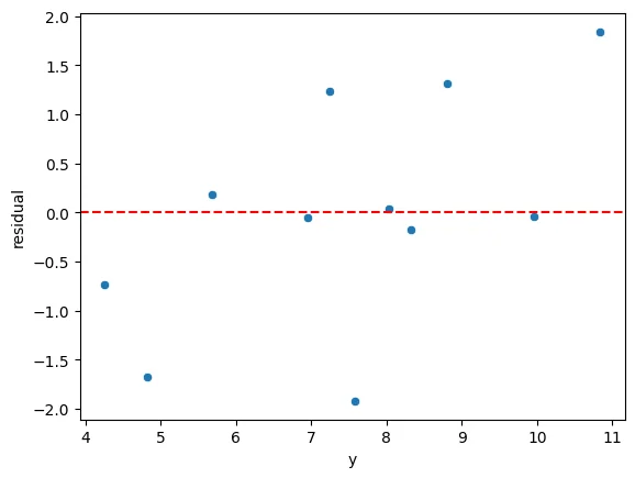
quartet = pd.read_csv('anscombes_quartet2.csv')quartet.columns = ['x','y']# y = 3.00 + 0.500x
quartet['pred_y'] = 3 + 0.5 * quartet['x']
quartet['residual'] = quartet['y'] - quartet['pred_y']
sns.scatterplot(data=quartet,x='x',y='y')
sns.lineplot(data=quartet,x='x',y='pred_y',color='red')
plt.vlines(quartet['x'],quartet['y'],quartet['y']-quartet['residual'])<Axes: xlabel='x', ylabel='y'>