00-Intro-to-Simple-Linear-Regression

Introduction to Simple Linear Regression

In this very simple example, we'll explore how to create a very simple fit line, the classic case of y=mx+b. We'll go carefully through each step, so you can see what type of question a simple fit line can answer. Keep in mind, this case is very simplified and is not the approach we'll take later on, its just here to get you thinking about linear regression in perhaps the same way Galton did.

Imports

Sample Data

This sample data is from ISLR. It displays sales (in thousands of units) for a particular product as a function of advertising budgets (in thousands of dollars) for TV, radio, and newspaper media.

python

df = pd.read_csv("Advertising.csv")

python

df.head()

Out · table

TV
radio
newspaper
sales
0

24 more lines

*Is there a relationship between total advertising spend and sales?*

python

df['total_spend'] = df['TV'] + df['radio'] + df['newspaper']

python

sns.scatterplot(x='total_spend',y='sales',data=df)

Out · result

<Axes: xlabel='total_spend', ylabel='sales'>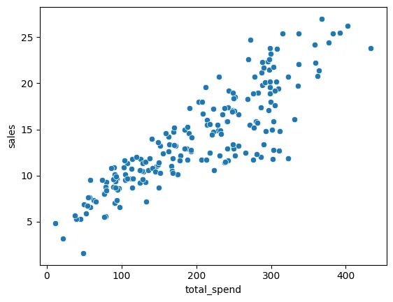

Least Squares Line

Full formulas available on Wikipedia: https://en.wikipedia.org/wiki/Linear_regression ,as well as in ISLR reading.

Understanding what a line of best fit answers. If someone was to spend a total of $200 , what would the expected sales be? We have simplified this quite a bit by combining all the features into "total spend", but we will come back to individual features later on. For now, let's focus on understanding what a linear regression line can help answer.

Our next ad campaign will have a total spend of $200, how many units do we expect to sell as a result of this?

python

# Basically, we want to figure out how to create this line
sns.regplot(x='total_spend',y='sales',data=df)

Out · result

<Axes: xlabel='total_spend', ylabel='sales'>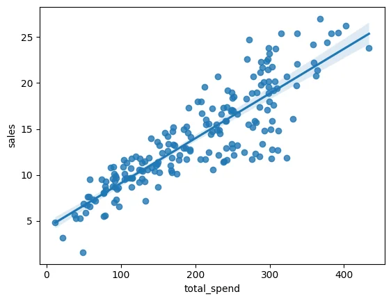

Let's go ahead and start solving: $y=mx+b$

Simply solve for m and b, remember, that as shown in the video, we are solving in a generalized form:

$\hat{y} = \beta_0 + \beta_1X$

Capitalized to signal that we are dealing with a matrix of values, we have a known matrix of labels (sales numbers) Y and a known matrix of total_spend (X). We are going to solve for the beta coefficients, which as we expand to more than just a single feature, will be important to build an understanding of what features have the most predictive power. We use y hat to indicate that y hat is a prediction or estimation, y would be a true label/known value.

We can use NumPy for this (if you really wanted to, you could solve this by hand)

python

X = df['total_spend']
y = df['sales']

python

help(np.polyfit)

Out · stdout

Help on _ArrayFunctionDispatcher in module numpy:

polyfit(x, y, deg, rcond=None, full=False, w=None, cov=False)
    Least squares polynomial fit.

170 more lines

    .. note::
       This forms part of the old polynomial API. Since version 1.4, the
       new polynomial API defined in `numpy.polynomial` is preferred.
       A summary of the differences can be found in the
       :doc:`transition guide </reference/routines.polynomials>`.

    Fit a polynomial ``p(x) = p[0] * x**deg + ... + p[deg]`` of degree `deg`
    to points `(x, y)`. Returns a vector of coefficients `p` that minimises
    the squared error in the order `deg`, `deg-1`, ... `0`.

    The `Polynomial.fit <numpy.polynomial.polynomial.Polynomial.fit>` class
    method is recommended for new code as it is more stable numerically. See
    the documentation of the method for more information.

    Parameters
    ----------
    x : array_like, shape (M,)
        x-coordinates of the M sample points ``(x[i], y[i])``.
    y : array_like, shape (M,) or (M, K)
        y-coordinates of the sample points. Several data sets of sample
        points sharing the same x-coordinates can be fitted at once by
        passing in a 2D-array that contains one dataset per column.
    deg : int
        Degree of the fitting polynomial
    rcond : float, optional
        Relative condition number of the fit. Singular values smaller than
        this relative to the largest singular value will be ignored. The
        default value is len(x)*eps, where eps is the relative precision of
        the float type, about 2e-16 in most cases.
    full : bool, optional
        Switch determining nature of return value. When it is False (the
        default) just the coefficients are returned, when True diagnostic
        information from the singular value decomposition is also returned.
    w : array_like, shape (M,), optional
        Weights. If not None, the weight ``w[i]`` applies to the unsquared
        residual ``y[i] - y_hat[i]`` at ``x[i]``. Ideally the weights are
        chosen so that the errors of the products ``w[i]*y[i]`` all have the
        same variance.  When using inverse-variance weighting, use
        ``w[i] = 1/sigma(y[i])``.  The default value is None.
    cov : bool or str, optional
        If given and not `False`, return not just the estimate but also its
        covariance matrix. By default, the covariance are scaled by
        chi2/dof, where dof = M - (deg + 1), i.e., the weights are presumed
        to be unreliable except in a relative sense and everything is scaled
        such that the reduced chi2 is unity. This scaling is omitted if
        ``cov='unscaled'``, as is relevant for the case that the weights are
        w = 1/sigma, with sigma known to be a reliable estimate of the
        uncertainty.

    Returns
    -------
    p : ndarray, shape (deg + 1,) or (deg + 1, K)
        Polynomial coefficients, highest power first.  If `y` was 2-D, the
        coefficients for `k`-th data set are in ``p[:,k]``.

    residuals, rank, singular_values, rcond
        These values are only returned if ``full == True``

        - residuals -- sum of squared residuals of the least squares fit
        - rank -- the effective rank of the scaled Vandermonde
           coefficient matrix
        - singular_values -- singular values of the scaled Vandermonde
           coefficient matrix
        - rcond -- value of `rcond`.

        For more details, see `numpy.linalg.lstsq`.

    V : ndarray, shape (deg + 1, deg + 1) or (deg + 1, deg + 1, K)
        Present only if ``full == False`` and ``cov == True``.  The covariance
        matrix of the polynomial coefficient estimates.  The diagonal of
        this matrix are the variance estimates for each coefficient.  If y
        is a 2-D array, then the covariance matrix for the `k`-th data set
        are in ``V[:,:,k]``


    Warns
    -----
    RankWarning
        The rank of the coefficient matrix in the least-squares fit is
        deficient. The warning is only raised if ``full == False``.

        The warnings can be turned off by

        >>> import warnings
        >>> warnings.simplefilter('ignore', np.exceptions.RankWarning)

    See Also
    --------
    polyval : Compute polynomial values.
    linalg.lstsq : Computes a least-squares fit.
    scipy.interpolate.UnivariateSpline : Computes spline fits.

    Notes
    -----
    The solution minimizes the squared error

    .. math::
        E = \sum_{j=0}^k |p(x_j) - y_j|^2

    in the equations::

        x[0]**n * p[0] + ... + x[0] * p[n-1] + p[n] = y[0]
        x[1]**n * p[0] + ... + x[1] * p[n-1] + p[n] = y[1]
        ...
        x[k]**n * p[0] + ... + x[k] * p[n-1] + p[n] = y[k]

    The coefficient matrix of the coefficients `p` is a Vandermonde matrix.

    `polyfit` issues a `~exceptions.RankWarning` when the least-squares fit is
    badly conditioned. This implies that the best fit is not well-defined due
    to numerical error. The results may be improved by lowering the polynomial
    degree or by replacing `x` by `x` - `x`.mean(). The `rcond` parameter
    can also be set to a value smaller than its default, but the resulting
    fit may be spurious: including contributions from the small singular
    values can add numerical noise to the result.

    Note that fitting polynomial coefficients is inherently badly conditioned
    when the degree of the polynomial is large or the interval of sample points
    is badly centered. The quality of the fit should always be checked in these
    cases. When polynomial fits are not satisfactory, splines may be a good
    alternative.

    References
    ----------
    .. [1] Wikipedia, "Curve fitting",
           https://en.wikipedia.org/wiki/Curve_fitting
    .. [2] Wikipedia, "Polynomial interpolation",
           https://en.wikipedia.org/wiki/Polynomial_interpolation

    Examples
    --------
    >>> import numpy as np
    >>> import warnings
    >>> x = np.array([0.0, 1.0, 2.0, 3.0,  4.0,  5.0])
    >>> y = np.array([0.0, 0.8, 0.9, 0.1, -0.8, -1.0])
    >>> z = np.polyfit(x, y, 3)
    >>> z
    array([ 0.08703704, -0.81349206,  1.69312169, -0.03968254]) # may vary

    It is convenient to use `poly1d` objects for dealing with polynomials:

    >>> p = np.poly1d(z)
    >>> p(0.5)
    0.6143849206349179 # may vary
    >>> p(3.5)
    -0.34732142857143039 # may vary
    >>> p(10)
    22.579365079365115 # may vary

    High-order polynomials may oscillate wildly:

    >>> with warnings.catch_warnings():
    ...     warnings.simplefilter('ignore', np.exceptions.RankWarning)
    ...     p30 = np.poly1d(np.polyfit(x, y, 30))
    ...
    >>> p30(4)
    -0.80000000000000204 # may vary
    >>> p30(5)
    -0.99999999999999445 # may vary
    >>> p30(4.5)
    -0.10547061179440398 # may vary

    Illustration:

    >>> import matplotlib.pyplot as plt
    >>> xp = np.linspace(-2, 6, 100)
    >>> _ = plt.plot(x, y, '.', xp, p(xp), '-', xp, p30(xp), '--')
    >>> plt.ylim(-2,2)
    (-2, 2)
    >>> plt.show()

python

# Returns highest order coef first!
np.polyfit(X,y,deg=1)

Out · result

array([-1.32539028e-09,  1.46034814e-06, -5.23540362e-04,  1.18664227e-01,
        1.51379069e+00])

python

# Potential Future Spend Budgets
potential_spend = np.linspace(0,500,100)

python

predicted_sales =  0.04868788*potential_spend + 4.24302822

python

plt.plot(potential_spend,predicted_sales)

Out · result

[<matplotlib.lines.Line2D at 0x11d5f7b30>]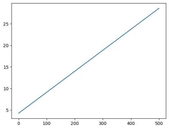

python

sns.scatterplot(x='total_spend',y='sales',data=df)
plt.plot(potential_spend,predicted_sales,color='red')

Out · result

[<matplotlib.lines.Line2D at 0x11d4f69c0>]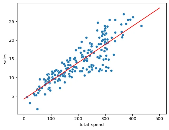

Our next ad campaign will have a total spend of $200, how many units do we expect to sell as a result of this?

python

spend = 200
predicted_sales =  0.04868788*spend + 4.24302822

python

predicted_sales

Out · result

13.98060422

Further considerations...which we will explore in much more depth!

Overfitting, Underfitting, and Measuring Performance

Notice we fit to order=1 , essentially a straight line, we can begin to explore higher orders, but does higher order mean an overall better fit? Is it possible to fit too much? Too little? How would we know and how do we even define a good fit?

python

np.polyfit(X,y,3)

Out · result

array([ 3.07615033e-07, -1.89392449e-04,  8.20886302e-02,  2.70495053e+00])

python

# Potential Future Spend Budgets
potential_spend = np.linspace(0,500,100)

python

predicted_sales =   3.07615033e-07*potential_spend**3 + -1.89392449e-04*potential_spend**2 + 8.20886302e-02*potential_spend**1 + 2.70495053e+00

python

sns.scatterplot(x='total_spend',y='sales',data=df)
plt.plot(potential_spend,predicted_sales,color='red')

Out · result

[<matplotlib.lines.Line2D at 0x11d4f4890>]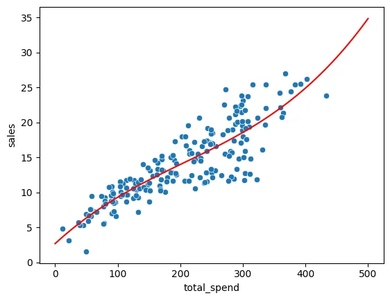

Is this better than our straight line fit? What are good ways of measuring this?

Multiple Features

The real data had 3 features, not everything in total spend, this would allow us to repeat the process and maybe get a more accurate result?

python

X = df[['TV','radio','newspaper']]
y = df['sales']

python

# Note here we're passing in 3 which matches up with 3 unique features, so we're not polynomial yet
np.polyfit(X,y,1)

Out · error

TypeError: expected 1D vector for x
---------------------------------------------------------------------------
TypeError                                 Traceback (most recent call last)
Cell In[36], line 2
      1 # Note here we're passing in 3 which matches up with 3 unique features, so we're not polynomial yet

10 more lines

----> 2 np.polyfit(X,y,1)

File ~/.pyenv/versions/3.12.6/lib/python3.12/site-packages/numpy/lib/_polynomial_impl.py:634, in polyfit(x, y, deg, rcond, full, w, cov)
    632     raise ValueError("expected deg >= 0")
    633 if x.ndim != 1:
--> 634     raise TypeError("expected 1D vector for x")
    635 if x.size == 0:
    636     raise TypeError("expected non-empty vector for x")

TypeError: expected 1D vector for x

Uh oh! Polyfit only works with a 1D X array! We'll need to move on to a more powerful library...