Linear Regression with SciKit-Learn
We saw how to create a very simple best fit line, but now let's greatly expand our toolkit to start thinking about the considerations of overfitting, underfitting, model evaluation, as well as multiple features!
Imports
Sample Data
This sample data is from ISLR. It displays sales (in thousands of units) for a particular product as a function of advertising budgets (in thousands of dollars) for TV, radio, and newspaper media.
df = pd.read_csv("Advertising.csv")df.head()TV
radio
newspaper
sales
024 more lines
230.1
37.8
69.2
22.1
1
44.5
39.3
45.1
10.4
2
17.2
45.9
69.3
9.3
3
151.5
41.3
58.5
18.5
4
180.8
10.8
58.4
12.9
Expanding the Questions
Previously, we explored *Is there a relationship between total advertising spend and sales*? as well as predicting the total sales for some value of total spend. Now we want to expand this to What is the relationship between each advertising channel (TV,Radio,Newspaper) and sales?
Multiple Features (N-Dimensional)
fig,axes = plt.subplots(nrows=1,ncols=3,figsize=(16,6))

axes[0].plot(df['TV'],df['sales'],'o')
axes[0].set_ylabel("Sales")
axes[0].set_title("TV Spend")

axes[1].plot(df['radio'],df['sales'],'o')
axes[1].set_title("Radio Spend")
axes[1].set_ylabel("Sales")

axes[2].plot(df['newspaper'],df['sales'],'o')
axes[2].set_title("Newspaper Spend");
axes[2].set_ylabel("Sales")
plt.tight_layout();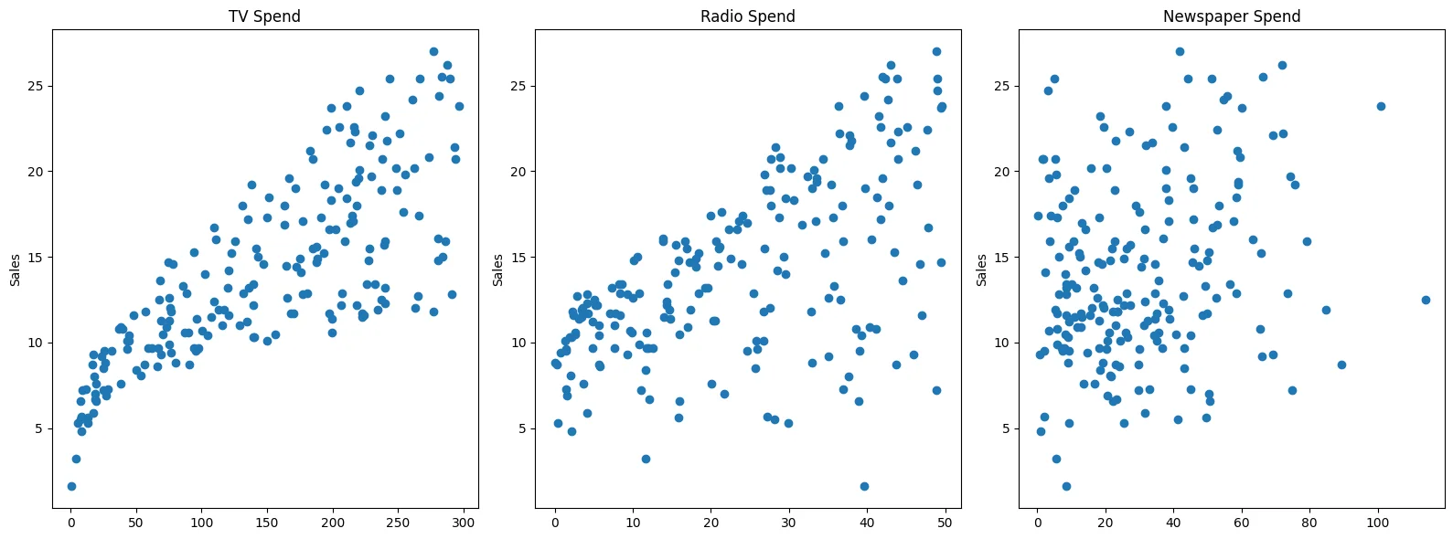
# Relationships between features
sns.pairplot(df,diag_kind='kde')<seaborn.axisgrid.PairGrid at 0x11eb6cb90>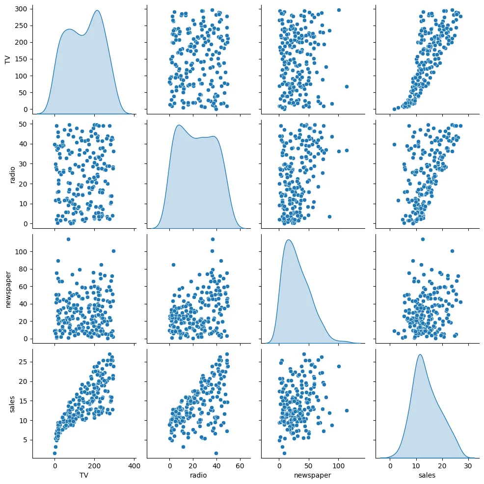
Introducing SciKit Learn
We will work a lot with the scitkit learn library, so get comfortable with its model estimator syntax, as well as exploring its incredibly useful documentation!
X = df.drop('sales',axis=1)
y = df['sales']
Train | Test Split
Make sure you have watched the Machine Learning Overview videos on Supervised Learning to understand why we do this step
from sklearn.model_selection import train_test_split# random_state:
# https://stackoverflow.com/questions/28064634/random-state-pseudo-random-number-in-scikit-learn
X_train, X_test, y_train, y_test = train_test_split(X, y, test_size=0.3, random_state=101)X_trainTV
radio
newspaper
85
193.243 more lines
18.4
65.7
183
287.6
43.0
71.8
127
80.2
0.0
9.2
53
182.6
46.2
58.7
100
222.4
4.3
49.8
...
...
...
...
63
102.7
29.6
8.4
70
199.1
30.6
38.7
81
239.8
4.1
36.9
11
214.7
24.0
4.0
95
163.3
31.6
52.9
140 rows × 3 columnsy_train85 15.2
183 26.2
127 8.8
53 21.2
100 11.77 more lines
       ...
63     14.0
70     18.3
81     12.3
11     17.4
95     16.9
Name: sales, Length: 140, dtype: float64X_testTV
radio
newspaper
37
74.7238 more lines
49.4
45.7
109
255.4
26.9
5.5
31
112.9
17.4
38.6
89
109.8
47.8
51.4
66
31.5
24.6
2.2
119
19.4
16.0
22.3
54
262.7
28.8
15.9
74
213.4
24.6
13.1
145
140.3
1.9
9.0
142
220.5
33.2
37.9
148
38.0
40.3
11.9
112
175.7
15.4
2.4
174
222.4
3.4
13.1
55
198.9
49.4
60.0
141
193.7
35.4
75.6
149
44.7
25.8
20.6
25
262.9
3.5
19.5
34
95.7
1.4
7.4
170
50.0
11.6
18.4
39
228.0
37.7
32.0
172
19.6
20.1
17.0
153
171.3
39.7
37.7
175
276.9
48.9
41.8
61
261.3
42.7
54.7
65
69.0
9.3
0.9
50
199.8
3.1
34.6
42
293.6
27.7
1.8
129
59.6
12.0
43.1
179
165.6
10.0
17.6
2
17.2
45.9
69.3
12
23.8
35.1
65.9
133
219.8
33.5
45.1
90
134.3
4.9
9.3
22
13.2
15.9
49.6
41
177.0
33.4
38.7
32
97.2
1.5
30.0
125
87.2
11.8
25.9
196
94.2
4.9
8.1
158
11.7
36.9
45.2
180
156.6
2.6
8.3
16
67.8
36.6
114.0
186
139.5
2.1
26.6
144
96.2
14.8
38.9
121
18.8
21.7
50.4
80
76.4
26.7
22.3
18
69.2
20.5
18.3
78
5.4
29.9
9.4
48
227.2
15.8
49.9
4
180.8
10.8
58.4
15
195.4
47.7
52.9
1
44.5
39.3
45.1
43
206.9
8.4
26.4
102
280.2
10.1
21.4
164
117.2
14.7
5.4
9
199.8
2.6
21.2
155
4.1
11.6
5.7
36
266.9
43.8
5.0
190
39.5
41.1
5.8
33
265.6
20.0
0.3
45
175.1
22.5
31.5y_test37 14.7
109 19.8
31 11.9
89 16.7
66 9.556 more lines
119     6.6
54     20.2
74     17.0
145    10.3
142    20.1
148    10.9
112    14.1
174    11.5
55     23.7
141    19.2
149    10.1
25     12.0
34      9.5
170     8.4
39     21.5
172     7.6
153    19.0
175    27.0
61     24.2
65      9.3
50     11.4
42     20.7
129     9.7
179    12.6
2       9.3
12      9.2
133    19.6
90     11.2
22      5.6
41     17.1
32      9.6
125    10.6
196     9.7
158     7.3
180    10.5
16     12.5
186    10.3
144    11.4
121     7.0
80     11.8
18     11.3
78      5.3
48     14.8
4      12.9
15     22.4
1      10.4
43     12.9
102    14.8
164    11.9
9      10.6
155     3.2
36     25.4
190    10.8
33     17.4
45     14.9
Name: sales, dtype: float64
Creating a Model (Estimator)
Import a model class from a model family
from sklearn.linear_model import LinearRegressionCreate an instance of the model with parameters
help(LinearRegression)Help on class LinearRegression in module sklearn.linear_model._base:
class LinearRegression(sklearn.base.MultiOutputMixin, sklearn.base.RegressorMixin, LinearModel)
| LinearRegression(*, fit_intercept=True, copy_X=True, tol=1e-06, n_jobs=None, positive=False)
|370 more lines
 |  Ordinary least squares Linear Regression.
 |
 |  LinearRegression fits a linear model with coefficients w = (w1, ..., wp)
 |  to minimize the residual sum of squares between the observed targets in
 |  the dataset, and the targets predicted by the linear approximation.
 |
 |  Parameters
 |  ----------
 |  fit_intercept : bool, default=True
 |      Whether to calculate the intercept for this model. If set
 |      to False, no intercept will be used in calculations
 |      (i.e. data is expected to be centered).
 |
 |  copy_X : bool, default=True
 |      If True, X will be copied; else, it may be overwritten.
 |
 |  tol : float, default=1e-6
 |      The precision of the solution (`coef_`) is determined by `tol` which
 |      specifies a different convergence criterion for the `lsqr` solver.
 |      `tol` is set as `atol` and `btol` of `scipy.sparse.linalg.lsqr` when
 |      fitting on sparse training data. This parameter has no effect when fitting
 |      on dense data.
 |
 |      .. versionadded:: 1.7
 |
 |  n_jobs : int, default=None
 |      The number of jobs to use for the computation. This will only provide
 |      speedup in case of sufficiently large problems, that is if firstly
 |      `n_targets > 1` and secondly `X` is sparse or if `positive` is set
 |      to `True`. ``None`` means 1 unless in a
 |      :obj:`joblib.parallel_backend` context. ``-1`` means using all
 |      processors. See :term:`Glossary <n_jobs>` for more details.
 |
 |  positive : bool, default=False
 |      When set to ``True``, forces the coefficients to be positive. This
 |      option is only supported for dense arrays.
 |
 |      For a comparison between a linear regression model with positive constraints
 |      on the regression coefficients and a linear regression without such constraints,
 |      see :ref:`sphx_glr_auto_examples_linear_model_plot_nnls.py`.
 |
 |      .. versionadded:: 0.24
 |
 |  Attributes
 |  ----------
 |  coef_ : array of shape (n_features, ) or (n_targets, n_features)
 |      Estimated coefficients for the linear regression problem.
 |      If multiple targets are passed during the fit (y 2D), this
 |      is a 2D array of shape (n_targets, n_features), while if only
 |      one target is passed, this is a 1D array of length n_features.
 |
 |  rank_ : int
 |      Rank of matrix `X`. Only available when `X` is dense.
 |
 |  singular_ : array of shape (min(X, y),)
 |      Singular values of `X`. Only available when `X` is dense.
 |
 |  intercept_ : float or array of shape (n_targets,)
 |      Independent term in the linear model. Set to 0.0 if
 |      `fit_intercept = False`.
 |
 |  n_features_in_ : int
 |      Number of features seen during :term:`fit`.
 |
 |      .. versionadded:: 0.24
 |
 |  feature_names_in_ : ndarray of shape (`n_features_in_`,)
 |      Names of features seen during :term:`fit`. Defined only when `X`
 |      has feature names that are all strings.
 |
 |      .. versionadded:: 1.0
 |
 |  See Also
 |  --------
 |  Ridge : Ridge regression addresses some of the
 |      problems of Ordinary Least Squares by imposing a penalty on the
 |      size of the coefficients with l2 regularization.
 |  Lasso : The Lasso is a linear model that estimates
 |      sparse coefficients with l1 regularization.
 |  ElasticNet : Elastic-Net is a linear regression
 |      model trained with both l1 and l2 -norm regularization of the
 |      coefficients.
 |
 |  Notes
 |  -----
 |  From the implementation point of view, this is just plain Ordinary
 |  Least Squares (scipy.linalg.lstsq) or Non Negative Least Squares
 |  (scipy.optimize.nnls) wrapped as a predictor object.
 |
 |  Examples
 |  --------
 |  >>> import numpy as np
 |  >>> from sklearn.linear_model import LinearRegression
 |  >>> X = np.array([[1, 1], [1, 2], [2, 2], [2, 3]])
 |  >>> # y = 1 * x_0 + 2 * x_1 + 3
 |  >>> y = np.dot(X, np.array([1, 2])) + 3
 |  >>> reg = LinearRegression().fit(X, y)
 |  >>> reg.score(X, y)
 |  1.0
 |  >>> reg.coef_
 |  array([1., 2.])
 |  >>> reg.intercept_
 |  np.float64(3.0)
 |  >>> reg.predict(np.array([[3, 5]]))
 |  array([16.])
 |
 |  Method resolution order:
 |      LinearRegression
 |      sklearn.base.MultiOutputMixin
 |      sklearn.base.RegressorMixin
 |      LinearModel
 |      sklearn.base.BaseEstimator
 |      sklearn.utils._repr_html.base.ReprHTMLMixin
 |      sklearn.utils._repr_html.base._HTMLDocumentationLinkMixin
 |      sklearn.utils._metadata_requests._MetadataRequester
 |      builtins.object
 |
 |  Methods defined here:
 |
 |  __init__(self, *, fit_intercept=True, copy_X=True, tol=1e-06, n_jobs=None, positive=False)
 |      Initialize self.  See help(type(self)) for accurate signature.
 |
 |  __sklearn_tags__(self)
 |
 |  fit(self, X, y, sample_weight=None)
 |      Fit linear model.
 |
 |      Parameters
 |      ----------
 |      X : {array-like, sparse matrix} of shape (n_samples, n_features)
 |          Training data.
 |
 |      y : array-like of shape (n_samples,) or (n_samples, n_targets)
 |          Target values. Will be cast to X's dtype if necessary.
 |
 |      sample_weight : array-like of shape (n_samples,), default=None
 |          Individual weights for each sample.
 |
 |          .. versionadded:: 0.17
 |             parameter *sample_weight* support to LinearRegression.
 |
 |      Returns
 |      -------
 |      self : object
 |          Fitted Estimator.
 |
 |  set_fit_request(self: sklearn.linear_model._base.LinearRegression, *, sample_weight: Union[bool, NoneType, str] = '$UNCHANGED$') -> sklearn.linear_model._base.LinearRegression from sklearn.utils._metadata_requests.RequestMethod.__get__.<locals>
 |      Configure whether metadata should be requested to be passed to the ``fit`` method.
 |
 |      Note that this method is only relevant when this estimator is used as a
 |      sub-estimator within a :term:`meta-estimator` and metadata routing is enabled
 |      with ``enable_metadata_routing=True`` (see :func:`sklearn.set_config`).
 |      Please check the :ref:`User Guide <metadata_routing>` on how the routing
 |      mechanism works.
 |
 |      The options for each parameter are:
 |
 |      - ``True``: metadata is requested, and passed to ``fit`` if provided. The request is ignored if metadata is not provided.
 |
 |      - ``False``: metadata is not requested and the meta-estimator will not pass it to ``fit``.
 |
 |      - ``None``: metadata is not requested, and the meta-estimator will raise an error if the user provides it.
 |
 |      - ``str``: metadata should be passed to the meta-estimator with this given alias instead of the original name.
 |
 |      The default (``sklearn.utils.metadata_routing.UNCHANGED``) retains the
 |      existing request. This allows you to change the request for some
 |      parameters and not others.
 |
 |      .. versionadded:: 1.3
 |
 |      Parameters
 |      ----------
 |      sample_weight : str, True, False, or None,                     default=sklearn.utils.metadata_routing.UNCHANGED
 |          Metadata routing for ``sample_weight`` parameter in ``fit``.
 |
 |      Returns
 |      -------
 |      self : object
 |          The updated object.
 |
 |  set_score_request(self: sklearn.linear_model._base.LinearRegression, *, sample_weight: Union[bool, NoneType, str] = '$UNCHANGED$') -> sklearn.linear_model._base.LinearRegression from sklearn.utils._metadata_requests.RequestMethod.__get__.<locals>
 |      Configure whether metadata should be requested to be passed to the ``score`` method.
 |
 |      Note that this method is only relevant when this estimator is used as a
 |      sub-estimator within a :term:`meta-estimator` and metadata routing is enabled
 |      with ``enable_metadata_routing=True`` (see :func:`sklearn.set_config`).
 |      Please check the :ref:`User Guide <metadata_routing>` on how the routing
 |      mechanism works.
 |
 |      The options for each parameter are:
 |
 |      - ``True``: metadata is requested, and passed to ``score`` if provided. The request is ignored if metadata is not provided.
 |
 |      - ``False``: metadata is not requested and the meta-estimator will not pass it to ``score``.
 |
 |      - ``None``: metadata is not requested, and the meta-estimator will raise an error if the user provides it.
 |
 |      - ``str``: metadata should be passed to the meta-estimator with this given alias instead of the original name.
 |
 |      The default (``sklearn.utils.metadata_routing.UNCHANGED``) retains the
 |      existing request. This allows you to change the request for some
 |      parameters and not others.
 |
 |      .. versionadded:: 1.3
 |
 |      Parameters
 |      ----------
 |      sample_weight : str, True, False, or None,                     default=sklearn.utils.metadata_routing.UNCHANGED
 |          Metadata routing for ``sample_weight`` parameter in ``score``.
 |
 |      Returns
 |      -------
 |      self : object
 |          The updated object.
 |
 |  ----------------------------------------------------------------------
 |  Data and other attributes defined here:
 |
 |  __abstractmethods__ = frozenset()
 |
 |  __annotations__ = {'_parameter_constraints': <class 'dict'>}
 |
 |  ----------------------------------------------------------------------
 |  Data descriptors inherited from sklearn.base.MultiOutputMixin:
 |
 |  __dict__
 |      dictionary for instance variables
 |
 |  __weakref__
 |      list of weak references to the object
 |
 |  ----------------------------------------------------------------------
 |  Methods inherited from sklearn.base.RegressorMixin:
 |
 |  score(self, X, y, sample_weight=None)
 |      Return :ref:`coefficient of determination <r2_score>` on test data.
 |
 |      The coefficient of determination, :math:`R^2`, is defined as
 |      :math:`(1 - \frac{u}{v})`, where :math:`u` is the residual
 |      sum of squares ``((y_true - y_pred)** 2).sum()`` and :math:`v`
 |      is the total sum of squares ``((y_true - y_true.mean()) ** 2).sum()``.
 |      The best possible score is 1.0 and it can be negative (because the
 |      model can be arbitrarily worse). A constant model that always predicts
 |      the expected value of `y`, disregarding the input features, would get
 |      a :math:`R^2` score of 0.0.
 |
 |      Parameters
 |      ----------
 |      X : array-like of shape (n_samples, n_features)
 |          Test samples. For some estimators this may be a precomputed
 |          kernel matrix or a list of generic objects instead with shape
 |          ``(n_samples, n_samples_fitted)``, where ``n_samples_fitted``
 |          is the number of samples used in the fitting for the estimator.
 |
 |      y : array-like of shape (n_samples,) or (n_samples, n_outputs)
 |          True values for `X`.
 |
 |      sample_weight : array-like of shape (n_samples,), default=None
 |          Sample weights.
 |
 |      Returns
 |      -------
 |      score : float
 |          :math:`R^2` of ``self.predict(X)`` w.r.t. `y`.
 |
 |      Notes
 |      -----
 |      The :math:`R^2` score used when calling ``score`` on a regressor uses
 |      ``multioutput='uniform_average'`` from version 0.23 to keep consistent
 |      with default value of :func:`~sklearn.metrics.r2_score`.
 |      This influences the ``score`` method of all the multioutput
 |      regressors (except for
 |      :class:`~sklearn.multioutput.MultiOutputRegressor`).
 |
 |  ----------------------------------------------------------------------
 |  Methods inherited from LinearModel:
 |
 |  predict(self, X)
 |      Predict using the linear model.
 |
 |      Parameters
 |      ----------
 |      X : array-like or sparse matrix, shape (n_samples, n_features)
 |          Samples.
 |
 |      Returns
 |      -------
 |      C : array, shape (n_samples,)
 |          Returns predicted values.
 |
 |  ----------------------------------------------------------------------
 |  Methods inherited from sklearn.base.BaseEstimator:
 |
 |  __getstate__(self)
 |      Helper for pickle.
 |
 |  __repr__(self, N_CHAR_MAX=700)
 |      Return repr(self).
 |
 |  __setstate__(self, state)
 |
 |  __sklearn_clone__(self)
 |
 |  get_params(self, deep=True)
 |      Get parameters for this estimator.
 |
 |      Parameters
 |      ----------
 |      deep : bool, default=True
 |          If True, will return the parameters for this estimator and
 |          contained subobjects that are estimators.
 |
 |      Returns
 |      -------
 |      params : dict
 |          Parameter names mapped to their values.
 |
 |  set_params(self, **params)
 |      Set the parameters of this estimator.
 |
 |      The method works on simple estimators as well as on nested objects
 |      (such as :class:`~sklearn.pipeline.Pipeline`). The latter have
 |      parameters of the form ``<component>__<parameter>`` so that it's
 |      possible to update each component of a nested object.
 |
 |      Parameters
 |      ----------
 |      **params : dict
 |          Estimator parameters.
 |
 |      Returns
 |      -------
 |      self : estimator instance
 |          Estimator instance.
 |
 |  ----------------------------------------------------------------------
 |  Methods inherited from sklearn.utils._metadata_requests._MetadataRequester:
 |
 |  get_metadata_routing(self)
 |      Get metadata routing of this object.
 |
 |      Please check :ref:`User Guide <metadata_routing>` on how the routing
 |      mechanism works.
 |
 |      Returns
 |      -------
 |      routing : MetadataRequest
 |          A :class:`~sklearn.utils.metadata_routing.MetadataRequest` encapsulating
 |          routing information.
 |
 |  ----------------------------------------------------------------------
 |  Class methods inherited from sklearn.utils._metadata_requests._MetadataRequester:
 |
 |  __init_subclass__(**kwargs)
 |      Set the ``set_{method}_request`` methods.
 |
 |      This uses PEP-487 [1]_ to set the ``set_{method}_request`` methods. It
 |      looks for the information available in the set default values which are
 |      set using ``__metadata_request__*`` class attributes, or inferred
 |      from method signatures.
 |
 |      The ``__metadata_request__*`` class attributes are used when a method
 |      does not explicitly accept a metadata through its arguments or if the
 |      developer would like to specify a request value for those metadata
 |      which are different from the default ``None``.
 |
 |      References
 |      ----------
| .. [1] https://www.python.org/dev/peps/pep-0487model = LinearRegression()Fit/Train the Model on the training data
Make sure you only fit to the training data, in order to fairly evaluate your model's performance on future data
model.fit(X_train,y_train)LinearRegression()In a Jupyter environment, please rerun this cell to show the HTML representation or trust the notebook.
On GitHub, the HTML representation is unable to render, please try loading this page with nbviewer.org.
LinearRegression
?Documentation for LinearRegressioniFitted
Parameters10 more lines
fit_intercept
True
copy_X
True
tol
1e-06
n_jobs
None
positive
False
Understanding and utilizing the Model
Evaluation on the Test Set
Metrics
Make sure you've viewed the video on these metrics! The three most common evaluation metrics for regression problems:
Mean Absolute Error (MAE) is the mean of the absolute value of the errors:
Mean Squared Error (MSE) is the mean of the squared errors:
Root Mean Squared Error (RMSE) is the square root of the mean of the squared errors:
Comparing these metrics:
- MAE is the easiest to understand, because it's the average error.
- MSE is more popular than MAE, because MSE "punishes" larger errors, which tends to be useful in the real world.
- RMSE is even more popular than MSE, because RMSE is interpretable in the "y" units.
All of these are loss functions, because we want to minimize them.
Calculate Performance on Test Set
We want to fairly evaluate our model, so we get performance metrics on the test set (data the model has never seen before).
# X_test# We only pass in test features
# The model predicts its own y hat
# We can then compare these results to the true y test label value
test_predictions = model.predict(X_test)test_predictionsarray([15.74131332, 19.61062568, 11.44888935, 17.00819787, 9.17285676,
7.01248287, 20.28992463, 17.29953992, 9.77584467, 19.22194224,
12.40503154, 13.89234998, 13.72541098, 21.28794031, 18.42456638,
9.98198406, 15.55228966, 7.68913693, 7.55614992, 20.40311209,
7.79215204, 18.24214098, 24.68631904, 22.82199068, 7.97962085,7 more lines
       12.65207264, 21.46925937,  8.05228573, 12.42315981, 12.50719678,
       10.77757812, 19.24460093, 10.070269  ,  6.70779999, 17.31492147,
        7.76764327,  9.25393336,  8.27834697, 10.58105585, 10.63591128,
       13.01002595,  9.77192057, 10.21469861,  8.04572042, 11.5671075 ,
       10.08368001,  8.99806574, 16.25388914, 13.23942315, 20.81493419,
       12.49727439, 13.96615898, 17.56285075, 11.14537013, 12.56261468,
5.50870279, 23.29465134, 12.62409688, 18.77399978, 15.18785675])from sklearn.metrics import mean_absolute_error,mean_squared_errorMAE = mean_absolute_error(y_test,test_predictions)
MSE = mean_squared_error(y_test,test_predictions)
RMSE = np.sqrt(MSE)MAE1.213745773614481MSE2.2987166978863796RMSE1.5161519375993884df['sales'].mean()14.0225Review our video to understand whether these values are "good enough".
Residuals
Revisiting Anscombe's Quartet: https://en.wikipedia.org/wiki/Anscombe%27s_quartet

quartet = pd.read_csv('anscombes_quartet1.csv')# y = 3.00 + 0.500x
quartet['pred_y'] = 3 + 0.5 * quartet['x']
quartet['residual'] = quartet['y'] - quartet['pred_y']
sns.scatterplot(data=quartet,x='x',y='y')
sns.lineplot(data=quartet,x='x',y='pred_y',color='red')
plt.vlines(quartet['x'],quartet['y'],quartet['y']-quartet['residual'])<matplotlib.collections.LineCollection at 0x21603321888>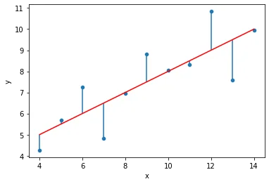
sns.kdeplot(quartet['residual'])<AxesSubplot:xlabel='residual', ylabel='Density'>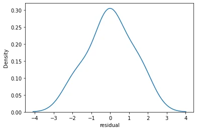
sns.scatterplot(data=quartet,x='y',y='residual')
plt.axhline(y=0, color='r', linestyle='--')<matplotlib.lines.Line2D at 0x216032d8a08>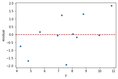
quartet = pd.read_csv('anscombes_quartet2.csv')quartet.columns = ['x','y']# y = 3.00 + 0.500x
quartet['pred_y'] = 3 + 0.5 * quartet['x']
quartet['residual'] = quartet['y'] - quartet['pred_y']
sns.scatterplot(data=quartet,x='x',y='y')
sns.lineplot(data=quartet,x='x',y='pred_y',color='red')
plt.vlines(quartet['x'],quartet['y'],quartet['y']-quartet['residual'])<matplotlib.collections.LineCollection at 0x21603475dc8>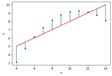
sns.kdeplot(quartet['residual'])<AxesSubplot:xlabel='residual', ylabel='Density'>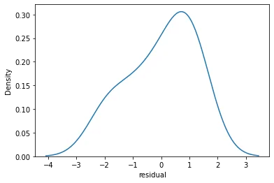
sns.scatterplot(data=quartet,x='y',y='residual')
plt.axhline(y=0, color='r', linestyle='--')<matplotlib.lines.Line2D at 0x21603410fc8>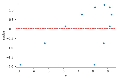
quartet = pd.read_csv('anscombes_quartet4.csv')quartetx
y
0
8.0
6.5830 more lines
1
8.0
5.76
2
8.0
7.71
3
8.0
8.84
4
8.0
8.47
5
8.0
7.04
6
8.0
5.25
7
19.0
12.50
8
8.0
5.56
9
8.0
7.91
10
8.0
6.89# y = 3.00 + 0.500x
quartet['pred_y'] = 3 + 0.5 * quartet['x']quartet['residual'] = quartet['y'] - quartet['pred_y']sns.scatterplot(data=quartet,x='x',y='y')
sns.lineplot(data=quartet,x='x',y='pred_y',color='red')
plt.vlines(quartet['x'],quartet['y'],quartet['y']-quartet['residual'])<matplotlib.collections.LineCollection at 0x216035bf808>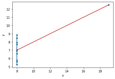
sns.kdeplot(quartet['residual'])<AxesSubplot:xlabel='residual', ylabel='Density'>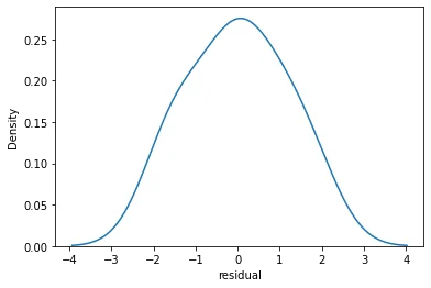
sns.scatterplot(data=quartet,x='y',y='residual')
plt.axhline(y=0, color='r', linestyle='--')<matplotlib.lines.Line2D at 0x21603641688>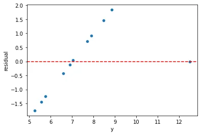
Plotting Residuals
It's also important to plot out residuals and check for normal distribution, this helps us understand if Linear Regression was a valid model choice.
# Predictions on training and testing sets
# Doing residuals separately will alert us to any issue with the split call
test_predictions = model.predict(X_test)# If our model was perfect, these would all be zeros
test_res = y_test - test_predictionssns.scatterplot(x=y_test,y=test_res)
plt.axhline(y=0, color='r', linestyle='--')<matplotlib.lines.Line2D at 0x216036b5308>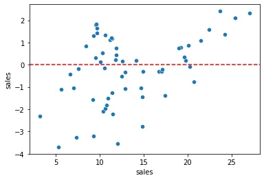
len(test_res)60sns.displot(test_res,bins=25,kde=True)<seaborn.axisgrid.FacetGrid at 0x2160370e708>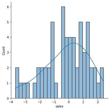
Still unsure if normality is a reasonable approximation? We can check against the normal probability plot.
# Create a figure and axis to plot on
fig, ax = plt.subplots(figsize=(6,8),dpi=100)
# probplot returns the raw values if needed
# we just want to see the plot, so we assign these values to _
_ = sp.stats.probplot(test_res,plot=ax)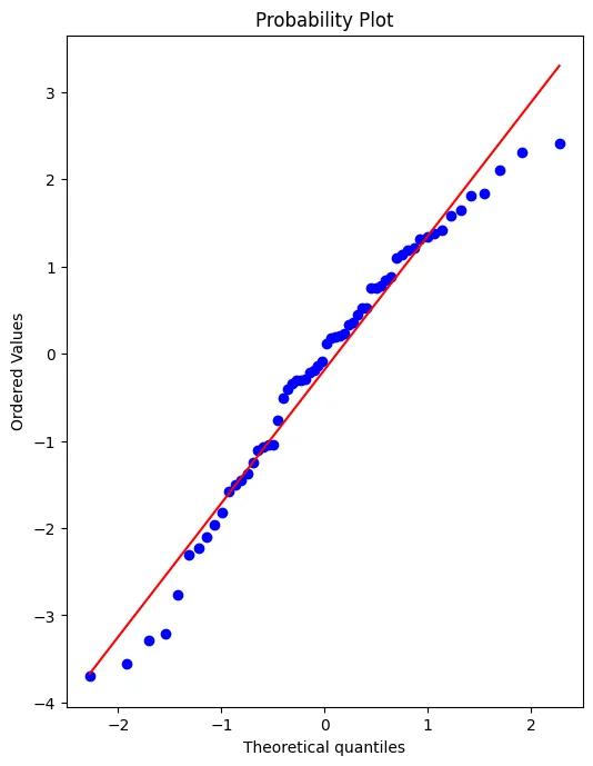
Retraining Model on Full Data
If we're satisfied with the performance on the test data, before deploying our model to the real world, we should retrain on all our data. (If we were not satisfied, we could update parameters or choose another model, something we'll discuss later on).
final_model = LinearRegression()final_model.fit(X,y)LinearRegression()Note how it may not really make sense to recalulate RMSE metrics here, since the model has already seen all the data, its not a fair judgement of performance to calculate RMSE on data its already seen, thus the purpose of the previous examination of test performance.
Deployment, Predictions, and Model Attributes
Final Model Fit
Note, we can only do this since we only have 3 features, for any more it becomes unreasonable.
y_hat = final_model.predict(X)fig,axes = plt.subplots(nrows=1,ncols=3,figsize=(16,6))
axes[0].plot(df['TV'],df['sales'],'o')
axes[0].plot(df['TV'],y_hat,'o',color='red')
axes[0].set_ylabel("Sales")
axes[0].set_title("TV Spend")
axes[1].plot(df['radio'],df['sales'],'o')
axes[1].plot(df['radio'],y_hat,'o',color='red')
axes[1].set_title("Radio Spend")
axes[1].set_ylabel("Sales")
axes[2].plot(df['newspaper'],df['sales'],'o')
axes[2].plot(df['radio'],y_hat,'o',color='red')
axes[2].set_title("Newspaper Spend");
axes[2].set_ylabel("Sales")
plt.tight_layout();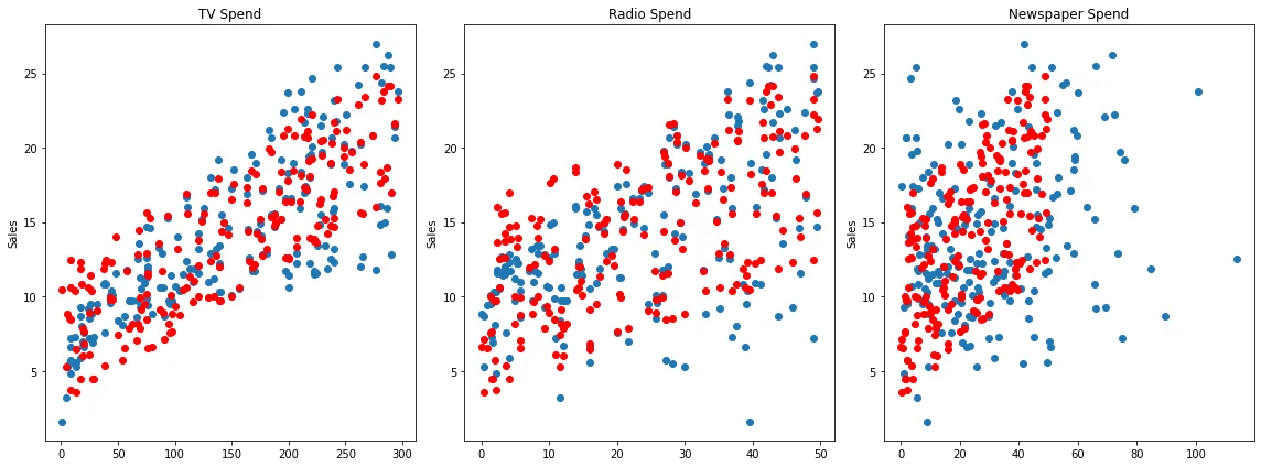
Residuals
Should be normally distributed as discussed in the video.
residuals = y_hat - ysns.scatterplot(x=y,y=residuals)
plt.axhline(y=0, color='r', linestyle='--')<matplotlib.lines.Line2D at 0x216039d7ac8>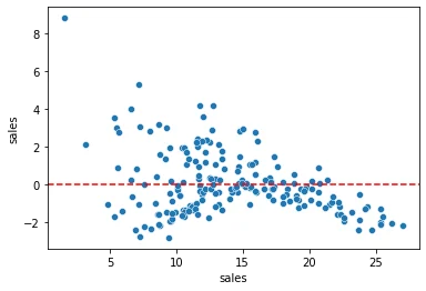
Coefficients
final_model.coef_array([ 0.04576465, 0.18853002, -0.00103749])coeff_df = pd.DataFrame(final_model.coef_,X.columns,columns=['Coefficient'])
coeff_dfCoefficient
TV
0.045765
radio
0.1885302 more lines
newspaper
-0.001037
Interpreting the coefficients:
- Holding all other features fixed, a 1 unit (A thousand dollars) increase in TV Spend is associated with an increase in sales of 0.045 "sales units", in this case 1000s of units .
- This basically means that for every $1000 dollars spend on TV Ads, we could expect 45 more units sold.
- Holding all other features fixed, a 1 unit (A thousand dollars) increase in Radio Spend is associated with an increase in sales of 0.188 "sales units", in this case 1000s of units .
- This basically means that for every $1000 dollars spend on Radio Ads, we could expect 188 more units sold.
- Holding all other features fixed, a 1 unit (A thousand dollars) increase in Newspaper Spend is associated with a decrease in sales of 0.001 "sales units", in this case 1000s of units .
- This basically means that for every $1000 dollars spend on Newspaper Ads, we could actually expect to sell 1 less unit. Being so close to 0, this heavily implies that newspaper spend has no real effect on sales.
*Note! In this case all our units were the same for each feature (1 unit = $1000 of ad spend). But in other datasets, units may not be the same, such as a housing dataset could try to predict a sale price with both a feature for number of bedrooms and a feature of total area like square footage. In this case it would make more sense to normalize the data, in order to clearly compare features and results. We will cover normalization later on.*
df.corr()TV
radio
newspaper
sales
TV19 more lines
1.000000
0.054809
0.056648
0.782224
radio
0.054809
1.000000
0.354104
0.576223
newspaper
0.056648
0.354104
1.000000
0.228299
sales
0.782224
0.576223
0.228299
1.000000
Prediction on New Data
Recall , X_test data set looks exactly the same as brand new data, so we simply need to call .predict() just as before to predict sales for a new advertising campaign.
Our next ad campaign will have a total spend of 149k on TV, 22k on Radio, and 12k on Newspaper Ads, how many units could we expect to sell as a result of this?
campaign = [[149,22,12]]final_model.predict(campaign)array([13.893032])How accurate is this prediction? No real way to know! We only know truly know our model's performance on the test data, that is why we had to be satisfied by it first, before training our full model
Model Persistence (Saving and Loading a Model)
from joblib import dump, loaddump(final_model, 'sales_model.joblib')['sales_model.joblib']loaded_model = load('sales_model.joblib')loaded_model.predict(campaign)array([13.893032])