Logistic Regression Project Exercise - Solutions
GOAL: Create a Classification Model that can predict whether or not a person has presence of heart disease based on physical features of that person (age,sex, cholesterol, etc...)
Complete the TASKs written in bold below.
Imports
TASK: Run the cell below to import the necessary libraries.
Data
This database contains 14 physical attributes based on physical testing of a patient. Blood samples are taken and the patient also conducts a brief exercise test. The "goal" field refers to the presence of heart disease in the patient. It is integer (0 for no presence, 1 for presence). In general, to confirm 100% if a patient has heart disease can be quite an invasive process, so if we can create a model that accurately predicts the likelihood of heart disease, we can help avoid expensive and invasive procedures.
Content
Attribute Information:
- age
- sex
- chest pain type (4 values)
- resting blood pressure
- serum cholestoral in mg/dl
- fasting blood sugar > 120 mg/dl
- resting electrocardiographic results (values 0,1,2)
- maximum heart rate achieved
- exercise induced angina
- oldpeak = ST depression induced by exercise relative to rest
- the slope of the peak exercise ST segment
- number of major vessels (0-3) colored by flourosopy
- thal: 3 = normal; 6 = fixed defect; 7 = reversable defect
- target:0 for no presence of heart disease, 1 for presence of heart disease
Original Source: https://archive.ics.uci.edu/ml/datasets/Heart+Disease
Creators:
Hungarian Institute of Cardiology. Budapest: Andras Janosi, M.D. University Hospital, Zurich, Switzerland: William Steinbrunn, M.D. University Hospital, Basel, Switzerland: Matthias Pfisterer, M.D. V.A. Medical Center, Long Beach and Cleveland Clinic Foundation: Robert Detrano, M.D., Ph.D.
TASK: Run the cell below to read in the data.
df = pd.read_csv('../DATA/heart.csv')df.head()age
sex
cp
trestbps
chol84 more lines
fbs
restecg
thalach
exang
oldpeak
slope
ca
thal
target
0
63
1
3
145
233
1
0
150
0
2.3
0
0
1
1
1
37
1
2
130
250
0
1
187
0
3.5
0
0
2
1
2
41
0
1
130
204
0
0
172
0
1.4
2
0
2
1
3
56
1
1
120
236
0
1
178
0
0.8
2
0
2
1
4
57
0
0
120
354
0
1
163
1
0.6
2
0
2
1df['target'].unique()array([1, 0], dtype=int64)Exploratory Data Analysis and Visualization
Feel free to explore the data further on your own.
TASK: Explore if the dataset has any missing data points and create a statistical summary of the numerical features as shown below.
# CODE HEREdf.info()<class 'pandas.core.frame.DataFrame'>
RangeIndex: 303 entries, 0 to 302
Data columns (total 14 columns):
# Column Non-Null Count Dtype
--- ------ -------------- ----- 16 more lines
 0   age       303 non-null    int64
 1   sex       303 non-null    int64
 2   cp        303 non-null    int64
 3   trestbps  303 non-null    int64
 4   chol      303 non-null    int64
 5   fbs       303 non-null    int64
 6   restecg   303 non-null    int64
 7   thalach   303 non-null    int64
 8   exang     303 non-null    int64
 9   oldpeak   303 non-null    float64
 10  slope     303 non-null    int64
 11  ca        303 non-null    int64
 12  thal      303 non-null    int64
 13  target    303 non-null    int64
dtypes: float64(1), int64(13)
memory usage: 33.3 KB# CODE HEREdf.describe().transpose()count
mean
std
min
25%129 more lines
50%
75%
max
age
303.0
54.366337
9.082101
29.0
47.5
55.0
61.0
77.0
sex
303.0
0.683168
0.466011
0.0
0.0
1.0
1.0
1.0
cp
303.0
0.966997
1.032052
0.0
0.0
1.0
2.0
3.0
trestbps
303.0
131.623762
17.538143
94.0
120.0
130.0
140.0
200.0
chol
303.0
246.264026
51.830751
126.0
211.0
240.0
274.5
564.0
fbs
303.0
0.148515
0.356198
0.0
0.0
0.0
0.0
1.0
restecg
303.0
0.528053
0.525860
0.0
0.0
1.0
1.0
2.0
thalach
303.0
149.646865
22.905161
71.0
133.5
153.0
166.0
202.0
exang
303.0
0.326733
0.469794
0.0
0.0
0.0
1.0
1.0
oldpeak
303.0
1.039604
1.161075
0.0
0.0
0.8
1.6
6.2
slope
303.0
1.399340
0.616226
0.0
1.0
1.0
2.0
2.0
ca
303.0
0.729373
1.022606
0.0
0.0
0.0
1.0
4.0
thal
303.0
2.313531
0.612277
0.0
2.0
2.0
3.0
3.0
target
303.0
0.544554
0.498835
0.0
0.0
1.0
1.0
1.0
Visualization Tasks
TASK: Create a bar plot that shows the total counts per target value.
# CODE HERE!sns.countplot(x='target',data=df)<AxesSubplot:xlabel='target', ylabel='count'>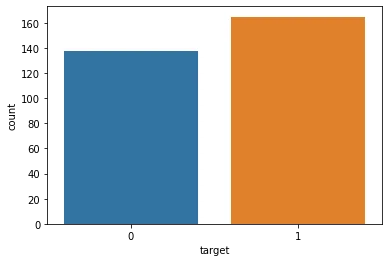
TASK: Create a pairplot that displays the relationships between the following columns:
['age','trestbps', 'chol','thalach','target']
Note: Running a pairplot on everything can take a very long time due to the number of features
# CODE HEREdf.columnsIndex(['age', 'sex', 'cp', 'trestbps', 'chol', 'fbs', 'restecg', 'thalach',
'exang', 'oldpeak', 'slope', 'ca', 'thal', 'target'],
dtype='object')# Running pairplot on everything will take a very long time to render!
sns.pairplot(df[['age','trestbps', 'chol','thalach','target']],hue='target')<seaborn.axisgrid.PairGrid at 0x2573c4e2148>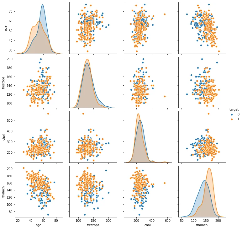
TASK: Create a heatmap that displays the correlation between all the columns.
# CODE HEREplt.figure(figsize=(12,8))
sns.heatmap(df.corr(),cmap='viridis',annot=True)<AxesSubplot:>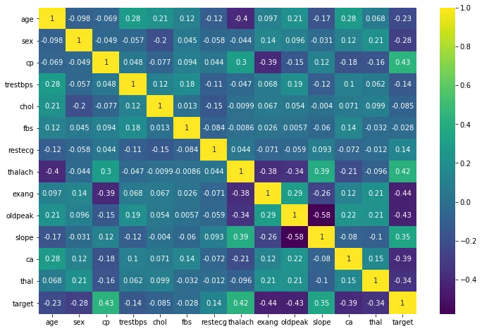
Machine Learning
Train | Test Split and Scaling
TASK: Separate the features from the labels into 2 objects, X and y.
# CODE HEREX = df.drop('target',axis=1)
y = df['target']TASK: Perform a train test split on the data, with the test size of 10% and a random_state of 101.
# CODE HEREfrom sklearn.model_selection import train_test_split
from sklearn.preprocessing import StandardScalerX_train, X_test, y_train, y_test = train_test_split(X, y, test_size=0.1, random_state=101)TASK: Create a StandardScaler object and normalize the X train and test set feature data. Make sure you only fit to the training data to avoid data leakage (data knowledge leaking from the test set).
# CODE HEREscaler = StandardScaler()scaled_X_train = scaler.fit_transform(X_train)
scaled_X_test = scaler.transform(X_test)Logistic Regression Model
*TASK: Create a Logistic Regression model and use Cross-Validation to find a well-performing C value for the hyper-parameter search. You have two options here, use LogisticRegressionCV OR use a combination of LogisticRegression and GridSearchCV. The choice is up to you, the solutions use the simpler LogisticRegressionCV approach.*
# CODE HEREfrom sklearn.linear_model import LogisticRegressionCV# help(LogisticRegressionCV)log_model = LogisticRegressionCV()log_model.fit(scaled_X_train,y_train)LogisticRegressionCV()TASK: Report back your search's optimal parameters, specifically the C value.
Note: You may get a different value than what is shown here depending on how you conducted your search.
# CODE HERElog_model.C_array([0.04641589])log_model.get_params(){'Cs': 10,
'class_weight': None,
'cv': None,
'dual': False,
'fit_intercept': True,12 more lines
 'intercept_scaling': 1.0,
 'l1_ratios': None,
 'max_iter': 100,
 'multi_class': 'auto',
 'n_jobs': None,
 'penalty': 'l2',
 'random_state': None,
 'refit': True,
 'scoring': None,
 'solver': 'lbfgs',
 'tol': 0.0001,
 'verbose': 0}
Coeffecients
TASK: Report back the model's coefficients.
log_model.coef_array([[-0.09621199, -0.39460154, 0.53534731, -0.13850191, -0.08830462,
0.02487341, 0.08083826, 0.29914053, -0.33438151, -0.352386 ,
0.25101033, -0.49735752, -0.37448551]])BONUS TASK: We didn't show this in the lecture notebooks, but you have the skills to do this! Create a visualization of the coefficients by using a barplot of their values. Even more bonus points if you can figure out how to sort the plot! If you get stuck on this, feel free to quickly view the solutions notebook for hints, there are many ways to do this, the solutions use a combination of pandas and seaborn.
#CODE HEREcoefs = pd.Series(index=X.columns,data=log_model.coef_[0])coefs = coefs.sort_values()plt.figure(figsize=(10,6))
sns.barplot(x=coefs.index,y=coefs.values);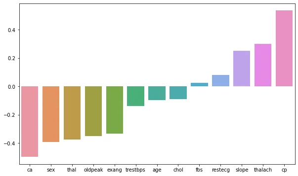
Model Performance Evaluation
TASK: Let's now evaluate your model on the remaining 10% of the data, the test set.
TASK: Create the following evaluations:
- Confusion Matrix Array
- Confusion Matrix Plot
- Classification Report
# CODE HEREfrom sklearn.metrics import confusion_matrix,classification_report,plot_confusion_matrixy_pred = log_model.predict(scaled_X_test)confusion_matrix(y_test,y_pred)array([[12, 3],
[ 2, 14]], dtype=int64)# CODE HEREplot_confusion_matrix(log_model,scaled_X_test,y_test)<sklearn.metrics._plot.confusion_matrix.ConfusionMatrixDisplay at 0x2573dba6e08>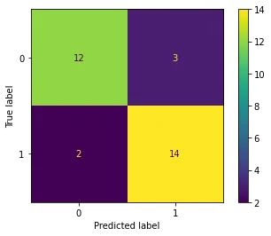
# CODE HEREprint(classification_report(y_test,y_pred)) precision recall f1-score support
0 0.86 0.80 0.83 15
1 0.82 0.88 0.85 16
3 more lines
    accuracy                           0.84        31
   macro avg       0.84      0.84      0.84        31
weighted avg       0.84      0.84      0.84        31
Performance Curves
TASK: Create both the precision recall curve and the ROC Curve.
from sklearn.metrics import plot_precision_recall_curve,plot_roc_curve# CODE HEREplot_precision_recall_curve(log_model,scaled_X_test,y_test)<sklearn.metrics._plot.precision_recall_curve.PrecisionRecallDisplay at 0x2573dc46cc8>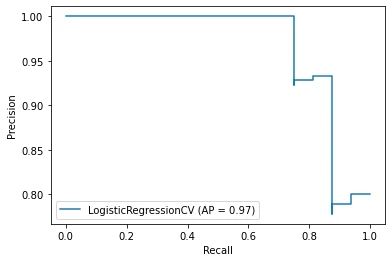
# CODE HEREplot_roc_curve(log_model,scaled_X_test,y_test)<sklearn.metrics._plot.roc_curve.RocCurveDisplay at 0x2573dc484c8>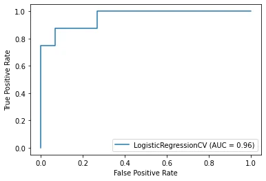
Final Task: A patient with the following features has come into the medical office:
age 48.0 sex 0.0 cp 2.0 trestbps 130.0 chol 275.0 fbs 0.0 restecg 1.0 thalach 139.0 exang 0.0 oldpeak 0.2 slope 2.0 ca 0.0 thal 2.0
TASK: What does your model predict for this patient? Do they have heart disease? How "sure" is your model of this prediction?
For convience, we created an array of the features for the patient above
patient = [[ 54. ,   1. ,   0. , 122. , 286. ,   0. ,   0. , 116. ,   1. ,
3.2, 1. , 2. , 2. ]]X_test.iloc[-1]age 54.0
sex 1.0
cp 0.0
trestbps 122.0
chol 286.09 more lines
fbs           0.0
restecg       0.0
thalach     116.0
exang         1.0
oldpeak       3.2
slope         1.0
ca            2.0
thal          2.0
Name: 268, dtype: float64y_test.iloc[-1]0log_model.predict(patient)array([0], dtype=int64)log_model.predict_proba(patient)array([[9.99999862e-01, 1.38455917e-07]])