Logistic Regression
Imports
Data
An experiment was conducted on 5000 participants to study the effects of age and physical health on hearing loss, specifically the ability to hear high pitched tones. This data displays the result of the study in which participants were evaluated and scored for physical ability and then had to take an audio test (pass/no pass) which evaluated their ability to hear high frequencies. The age of the user was also noted. Is it possible to build a model that would predict someone's liklihood to hear the high frequency sound based solely on their features (age and physical score)?
- Features
- age - Age of participant in years
- physical_score - Score achieved during physical exam
- Label/Target
- test_result - 0 if no pass, 1 if test passed
df = pd.read_csv('../DATA/hearing_test.csv')df.head()age
physical_score
test_result
0
33.018 more lines
40.7
1
1
50.0
37.2
1
2
52.0
24.7
0
3
56.0
31.0
0
4
35.0
42.9
1
Exploratory Data Analysis and Visualization
Feel free to explore the data further on your own.
df.info()<class 'pandas.core.frame.DataFrame'>
RangeIndex: 5000 entries, 0 to 4999
Data columns (total 3 columns):
# Column Non-Null Count Dtype
--- ------ -------------- ----- 5 more lines
 0   age             5000 non-null   float64
 1   physical_score  5000 non-null   float64
 2   test_result     5000 non-null   int64
dtypes: float64(2), int64(1)
memory usage: 117.3 KBdf.describe()age
physical_score
test_result
count
5000.00000030 more lines
5000.000000
5000.000000
mean
51.609000
32.760260
0.600000
std
11.287001
8.169802
0.489947
min
18.000000
-0.000000
0.000000
25%
43.000000
26.700000
0.000000
50%
51.000000
35.300000
1.000000
75%
60.000000
38.900000
1.000000
max
90.000000
50.000000
1.000000df['test_result'].value_counts()1 3000
0 2000
Name: test_result, dtype: int64sns.countplot(data=df,x='test_result')<AxesSubplot:xlabel='test_result', ylabel='count'>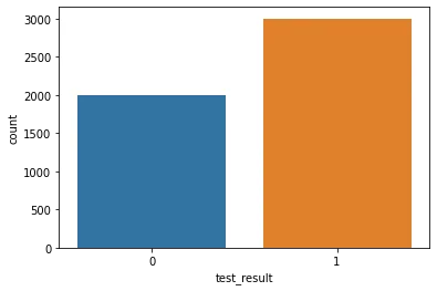
sns.boxplot(x='test_result',y='age',data=df)<AxesSubplot:xlabel='test_result', ylabel='age'>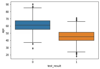
sns.boxplot(x='test_result',y='physical_score',data=df)<AxesSubplot:xlabel='test_result', ylabel='physical_score'>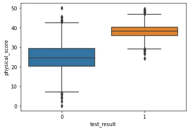
sns.scatterplot(x='age',y='physical_score',data=df,hue='test_result')<AxesSubplot:xlabel='age', ylabel='physical_score'>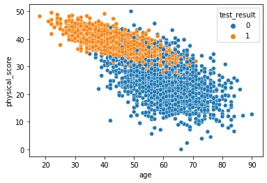
sns.pairplot(df,hue='test_result')<seaborn.axisgrid.PairGrid at 0x19ceae2fd08>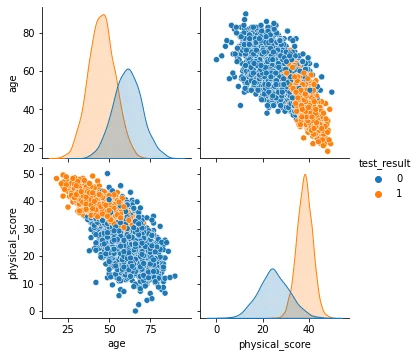
sns.heatmap(df.corr(),annot=True)<AxesSubplot:>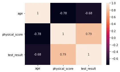
sns.scatterplot(x='physical_score',y='test_result',data=df)<AxesSubplot:xlabel='physical_score', ylabel='test_result'>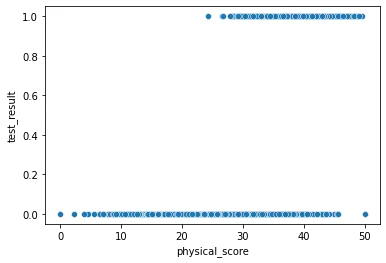
sns.scatterplot(x='age',y='test_result',data=df)<AxesSubplot:xlabel='age', ylabel='test_result'>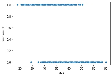
Easily discover new plot types with a google search! Searching for "3d matplotlib scatter plot" quickly takes you to: https://matplotlib.org/3.1.1/gallery/mplot3d/scatter3d.html
from mpl_toolkits.mplot3d import Axes3D
fig = plt.figure()
ax = fig.add_subplot(111, projection='3d')
ax.scatter(df['age'],df['physical_score'],df['test_result'],c=df['test_result'])<mpl_toolkits.mplot3d.art3d.Path3DCollection at 0x19ceaf878c8>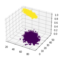
Train | Test Split and Scaling
X = df.drop('test_result',axis=1)
y = df['test_result']from sklearn.model_selection import train_test_split
from sklearn.preprocessing import StandardScalerX_train, X_test, y_train, y_test = train_test_split(X, y, test_size=0.1, random_state=101)scaler = StandardScaler()scaled_X_train = scaler.fit_transform(X_train)
scaled_X_test = scaler.transform(X_test)Logistic Regression Model
from sklearn.linear_model import LogisticRegression# help(LogisticRegression)# help(LogisticRegressionCV)log_model = LogisticRegression()log_model.fit(scaled_X_train,y_train)LogisticRegression()Coefficient Interpretation
Things to remember:
- These coeffecients relate to the odds and can not be directly interpreted as in linear regression.
- We trained on a scaled version of the data
- It is much easier to understand and interpret the relationship between the coefficients than it is to interpret the coefficients relationship with the probability of the target/label class.
Make sure to watch the video explanation, also check out the links below:
- https://stats.idre.ucla.edu/stata/faq/how-do-i-interpret-odds-ratios-in-logistic-regression/
- https://stats.idre.ucla.edu/other/mult-pkg/faq/general/faq-how-do-i-interpret-odds-ratios-in-logistic-regression/
The odds ratio
For a continuous independent variable the odds ratio can be defined as:

This exponential relationship provides an interpretation for
The odds multiply by for every 1-unit increase in x.
log_model.coef_array([[-0.94953524, 3.45991194]])This means:
- We can expect the odds of passing the test to decrease (the original coeff was negative) per unit increase of the age.
- We can expect the odds of passing the test to increase (the original coeff was positive) per unit increase of the physical score.
- Based on the ratios with each other, the physical_score indicator is a stronger predictor than age.
Model Performance on Classification Tasks
from sklearn.metrics import accuracy_score,confusion_matrix,classification_report,plot_confusion_matrixy_pred = log_model.predict(scaled_X_test)accuracy_score(y_test,y_pred)0.93confusion_matrix(y_test,y_pred)array([[172, 21],
[ 14, 293]], dtype=int64)plot_confusion_matrix(log_model,scaled_X_test,y_test)<sklearn.metrics._plot.confusion_matrix.ConfusionMatrixDisplay at 0x19ceb65e588>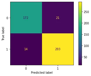
# Scaled so highest value=1
plot_confusion_matrix(log_model,scaled_X_test,y_test,normalize='true')<sklearn.metrics._plot.confusion_matrix.ConfusionMatrixDisplay at 0x19ceb691b88>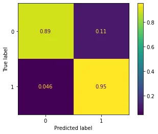
print(classification_report(y_test,y_pred)) precision recall f1-score support
0 0.92 0.89 0.91 193
1 0.93 0.95 0.94 307
3 more lines
    accuracy                           0.93       500
   macro avg       0.93      0.92      0.93       500
weighted avg 0.93 0.93 0.93 500X_train.iloc[0]age 32.0
physical_score 43.0
Name: 141, dtype: float64y_train.iloc[0]1# 0% probability of 0 class
# 100% probability of 1 class
log_model.predict_proba(X_train.iloc[0].values.reshape(1, -1))array([[0., 1.]])log_model.predict(X_train.iloc[0].values.reshape(1, -1))array([1], dtype=int64)Evaluating Curves and AUC
Make sure to watch the video on this!
from sklearn.metrics import precision_recall_curve,plot_precision_recall_curve,plot_roc_curveplot_precision_recall_curve(log_model,scaled_X_test,y_test)<sklearn.metrics._plot.precision_recall_curve.PrecisionRecallDisplay at 0x19cec76dac8>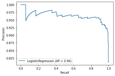
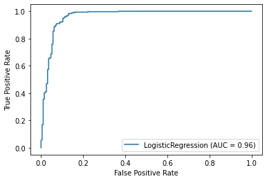
plot_roc_curve(log_model,scaled_X_test,y_test)<sklearn.metrics._plot.roc_curve.RocCurveDisplay at 0x19ceb5c4288>