Multi-Class Logistic Regression
Students often ask how to perform non binary classification with Logistic Regression. Fortunately, the process with scikit-learn is pretty much the same as with binary classification. To expand our understanding, we'll go through a simple data set, as well as seeing how to use LogisiticRegression with a manual GridSearchCV (instead of LogisticRegressionCV).
Imports
Data
We will work with the classic Iris Data Set. The Iris flower data set or Fisher's Iris data set is a multivariate data set introduced by the British statistician, eugenicist, and biologist Ronald Fisher in his 1936 paper The use of multiple measurements in taxonomic problems as an example of linear discriminant analysis.
Full Details: https://en.wikipedia.org/wiki/Iris_flower_data_set
df = pd.read_csv('../DATA/iris.csv')df.head()sepal_length
sepal_width
petal_length
petal_width
species30 more lines
0
5.1
3.5
1.4
0.2
setosa
1
4.9
3.0
1.4
0.2
setosa
2
4.7
3.2
1.3
0.2
setosa
3
4.6
3.1
1.5
0.2
setosa
4
5.0
3.6
1.4
0.2
setosa
Exploratory Data Analysis and Visualization
Feel free to explore the data further on your own.
df.info()<class 'pandas.core.frame.DataFrame'>
RangeIndex: 150 entries, 0 to 149
Data columns (total 5 columns):
# Column Non-Null Count Dtype
--- ------ -------------- ----- 7 more lines
 0   sepal_length  150 non-null    float64
 1   sepal_width   150 non-null    float64
 2   petal_length  150 non-null    float64
 3   petal_width   150 non-null    float64
 4   species       150 non-null    object
dtypes: float64(4), object(1)
memory usage: 6.0+ KBdf.describe()sepal_length
sepal_width
petal_length
petal_width
count39 more lines
150.000000
150.000000
150.000000
150.000000
mean
5.843333
3.054000
3.758667
1.198667
std
0.828066
0.433594
1.764420
0.763161
min
4.300000
2.000000
1.000000
0.100000
25%
5.100000
2.800000
1.600000
0.300000
50%
5.800000
3.000000
4.350000
1.300000
75%
6.400000
3.300000
5.100000
1.800000
max
7.900000
4.400000
6.900000
2.500000df['species'].value_counts()setosa 50
versicolor 50
virginica 50
Name: species, dtype: int64sns.countplot(df['species'])<AxesSubplot:xlabel='species', ylabel='count'>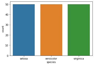
sns.scatterplot(x='sepal_length',y='sepal_width',data=df,hue='species')<AxesSubplot:xlabel='sepal_length', ylabel='sepal_width'>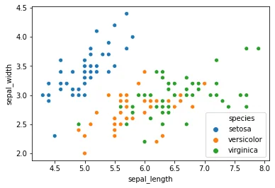
sns.scatterplot(x='petal_length',y='petal_width',data=df,hue='species')<AxesSubplot:xlabel='petal_length', ylabel='petal_width'>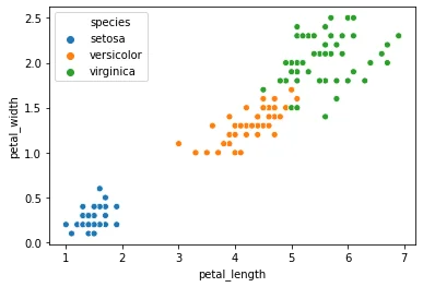
sns.pairplot(df,hue='species')<seaborn.axisgrid.PairGrid at 0x2a1a26a4908>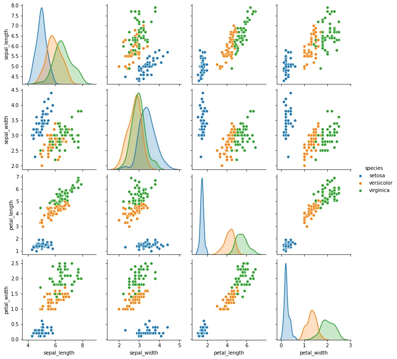
sns.heatmap(df.corr(),annot=True)<AxesSubplot:>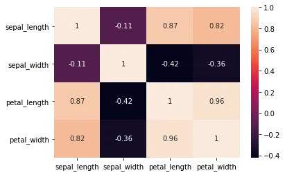
Easily discover new plot types with a google search! Searching for "3d matplotlib scatter plot" quickly takes you to: https://matplotlib.org/3.1.1/gallery/mplot3d/scatter3d.html
df['species'].unique()array(['setosa', 'versicolor', 'virginica'], dtype=object)from mpl_toolkits.mplot3d import Axes3D
fig = plt.figure()
ax = fig.add_subplot(111, projection='3d')
colors = df['species'].map({'setosa':0, 'versicolor':1, 'virginica':2})
ax.scatter(df['sepal_width'],df['petal_width'],df['petal_length'],c=colors);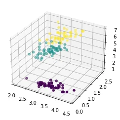
Train | Test Split and Scaling
X = df.drop('species',axis=1)
y = df['species']from sklearn.model_selection import train_test_split
from sklearn.preprocessing import StandardScalerX_train, X_test, y_train, y_test = train_test_split(X, y, test_size=0.25, random_state=101)scaler = StandardScaler()scaled_X_train = scaler.fit_transform(X_train)
scaled_X_test = scaler.transform(X_test)Multi-Class Logistic Regression Model
from sklearn.linear_model import LogisticRegressionfrom sklearn.model_selection import GridSearchCV# Depending on warnings you may need to adjust max iterations allowed
# Or experiment with different solvers
log_model = LogisticRegression(solver='saga',multi_class="ovr",max_iter=5000)GridSearch for Best Hyper-Parameters
Main parameter choices are regularization penalty choice and regularization C value.
# Penalty Type
penalty = ['l1', 'l2']

# Use logarithmically spaced C values (recommended in official docs)
C = np.logspace(0, 4, 10)grid_model = GridSearchCV(log_model,param_grid={'C':C,'penalty':penalty})grid_model.fit(scaled_X_train,y_train)GridSearchCV(estimator=LogisticRegression(max_iter=5000, multi_class='ovr',
solver='saga'),
param_grid={'C': array([1.00000000e+00, 2.78255940e+00, 7.74263683e+00, 2.15443469e+01,
5.99484250e+01, 1.66810054e+02, 4.64158883e+02, 1.29154967e+03,
3.59381366e+03, 1.00000000e+04]),1 more line
'penalty': ['l1', 'l2']})grid_model.best_params_{'C': 7.742636826811269, 'penalty': 'l1'}Model Performance on Classification Tasks
from sklearn.metrics import accuracy_score,confusion_matrix,classification_report,plot_confusion_matrixy_pred = grid_model.predict(scaled_X_test)accuracy_score(y_test,y_pred)0.9736842105263158confusion_matrix(y_test,y_pred)array([[10, 0, 0],
[ 0, 17, 0],
[ 0, 1, 10]], dtype=int64)plot_confusion_matrix(grid_model,scaled_X_test,y_test)<sklearn.metrics._plot.confusion_matrix.ConfusionMatrixDisplay at 0x2a1a83ac0c8>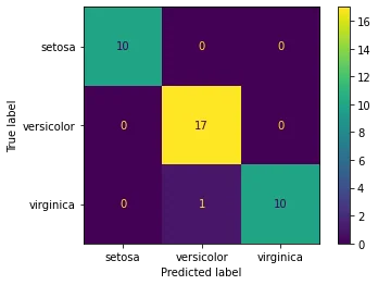
# Scaled so highest value=1
plot_confusion_matrix(grid_model,scaled_X_test,y_test,normalize='true')<sklearn.metrics._plot.confusion_matrix.ConfusionMatrixDisplay at 0x2a1a843ac48>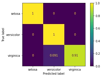
print(classification_report(y_test,y_pred)) precision recall f1-score support
setosa 1.00 1.00 1.00 10
versicolor 0.94 1.00 0.97 17
virginica 1.00 0.91 0.95 114 more lines
    accuracy                           0.97        38
   macro avg       0.98      0.97      0.97        38
weighted avg       0.98      0.97      0.97        38
Evaluating Curves and AUC
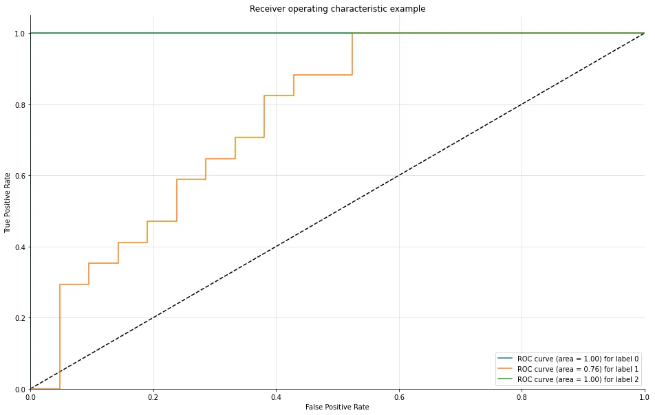
Make sure to watch the video on this! We need to manually create the plots for a Multi-Class situation. Fortunately, Scikit-learn's documentation already has plenty of examples on this.
Source: https://scikit-learn.org/stable/auto_examples/model_selection/plot_roc.html
We have created a function for you that does this automatically, essentially creating and plotting an ROC per class.
from sklearn.metrics import roc_curve, aucdef plot_multiclass_roc(clf, X_test, y_test, n_classes, figsize=(5,5)):
y_score = clf.decision_function(X_test)
# structures
fpr = dict()
tpr = dict()
roc_auc = dict()
# calculate dummies once
y_test_dummies = pd.get_dummies(y_test, drop_first=False).values
for i in range(n_classes):
fpr[i], tpr[i], _ = roc_curve(y_test_dummies[:, i], y_score[:, i])
roc_auc[i] = auc(fpr[i], tpr[i])
# roc for each class
fig, ax = plt.subplots(figsize=figsize)
ax.plot([0, 1], [0, 1], 'k--')
ax.set_xlim([0.0, 1.0])
ax.set_ylim([0.0, 1.05])
ax.set_xlabel('False Positive Rate')
ax.set_ylabel('True Positive Rate')
ax.set_title('Receiver operating characteristic example')
for i in range(n_classes):
ax.plot(fpr[i], tpr[i], label='ROC curve (area = %0.2f) for label %i' % (roc_auc[i], i))
ax.legend(loc="best")
ax.grid(alpha=.4)
sns.despine()
plt.show()plot_multiclass_roc(grid_model, scaled_X_test, y_test, n_classes=3, figsize=(16, 10))