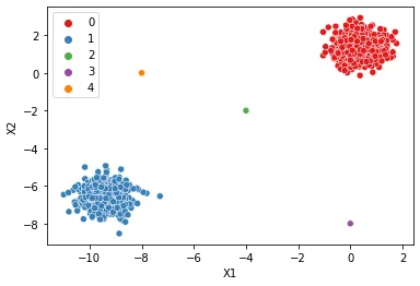
DBSCAN Hyperparameters
Let's explore the hyperparameters for DBSCAN and how they can change results!
DBSCAN and Clustering Examples
two_blobs = pd.read_csv('../DATA/cluster_two_blobs.csv')
two_blobs_outliers = pd.read_csv('../DATA/cluster_two_blobs_outliers.csv')sns.scatterplot(data=two_blobs,x='X1',y='X2')<AxesSubplot:xlabel='X1', ylabel='X2'>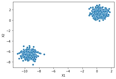
# plt.figure(figsize=(10,6),dpi=200)
sns.scatterplot(data=two_blobs_outliers,x='X1',y='X2')<AxesSubplot:xlabel='X1', ylabel='X2'>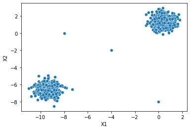
Label Discovery
def display_categories(model,data):
    labels = model.fit_predict(data)
    sns.scatterplot(data=data,x='X1',y='X2',hue=labels,palette='Set1')
DBSCAN
from sklearn.cluster import DBSCANhelp(DBSCAN)Help on class DBSCAN in module sklearn.cluster._dbscan:
class DBSCAN(sklearn.base.ClusterMixin, sklearn.base.BaseEstimator)
| DBSCAN(eps=0.5, *, min_samples=5, metric='euclidean', metric_params=None, algorithm='auto', leaf_size=30, p=None, n_jobs=None)
| 232 more lines
 |  Perform DBSCAN clustering from vector array or distance matrix.
 |
 |  DBSCAN - Density-Based Spatial Clustering of Applications with Noise.
 |  Finds core samples of high density and expands clusters from them.
 |  Good for data which contains clusters of similar density.
 |
 |  Read more in the :ref:`User Guide <dbscan>`.
 |
 |  Parameters
 |  ----------
 |  eps : float, default=0.5
 |      The maximum distance between two samples for one to be considered
 |      as in the neighborhood of the other. This is not a maximum bound
 |      on the distances of points within a cluster. This is the most
 |      important DBSCAN parameter to choose appropriately for your data set
 |      and distance function.
 |
 |  min_samples : int, default=5
 |      The number of samples (or total weight) in a neighborhood for a point
 |      to be considered as a core point. This includes the point itself.
 |
 |  metric : string, or callable, default='euclidean'
 |      The metric to use when calculating distance between instances in a
 |      feature array. If metric is a string or callable, it must be one of
 |      the options allowed by :func:`sklearn.metrics.pairwise_distances` for
 |      its metric parameter.
 |      If metric is "precomputed", X is assumed to be a distance matrix and
 |      must be square. X may be a :term:`Glossary <sparse graph>`, in which
 |      case only "nonzero" elements may be considered neighbors for DBSCAN.
 |
 |      .. versionadded:: 0.17
 |         metric *precomputed* to accept precomputed sparse matrix.
 |
 |  metric_params : dict, default=None
 |      Additional keyword arguments for the metric function.
 |
 |      .. versionadded:: 0.19
 |
 |  algorithm : {'auto', 'ball_tree', 'kd_tree', 'brute'}, default='auto'
 |      The algorithm to be used by the NearestNeighbors module
 |      to compute pointwise distances and find nearest neighbors.
 |      See NearestNeighbors module documentation for details.
 |
 |  leaf_size : int, default=30
 |      Leaf size passed to BallTree or cKDTree. This can affect the speed
 |      of the construction and query, as well as the memory required
 |      to store the tree. The optimal value depends
 |      on the nature of the problem.
 |
 |  p : float, default=None
 |      The power of the Minkowski metric to be used to calculate distance
 |      between points.
 |
 |  n_jobs : int, default=None
 |      The number of parallel jobs to run.
 |      ``None`` means 1 unless in a :obj:`joblib.parallel_backend` context.
 |      ``-1`` means using all processors. See :term:`Glossary <n_jobs>`
 |      for more details.
 |
 |  Attributes
 |  ----------
 |  core_sample_indices_ : ndarray of shape (n_core_samples,)
 |      Indices of core samples.
 |
 |  components_ : ndarray of shape (n_core_samples, n_features)
 |      Copy of each core sample found by training.
 |
 |  labels_ : ndarray of shape (n_samples)
 |      Cluster labels for each point in the dataset given to fit().
 |      Noisy samples are given the label -1.
 |
 |  Examples
 |  --------
 |  >>> from sklearn.cluster import DBSCAN
 |  >>> import numpy as np
 |  >>> X = np.array([[1, 2], [2, 2], [2, 3],
 |  ...               [8, 7], [8, 8], [25, 80]])
 |  >>> clustering = DBSCAN(eps=3, min_samples=2).fit(X)
 |  >>> clustering.labels_
 |  array([ 0,  0,  0,  1,  1, -1])
 |  >>> clustering
 |  DBSCAN(eps=3, min_samples=2)
 |
 |  See also
 |  --------
 |  OPTICS
 |      A similar clustering at multiple values of eps. Our implementation
 |      is optimized for memory usage.
 |
 |  Notes
 |  -----
 |  For an example, see :ref:`examples/cluster/plot_dbscan.py
 |  <sphx_glr_auto_examples_cluster_plot_dbscan.py>`.
 |
 |  This implementation bulk-computes all neighborhood queries, which increases
 |  the memory complexity to O(n.d) where d is the average number of neighbors,
 |  while original DBSCAN had memory complexity O(n). It may attract a higher
 |  memory complexity when querying these nearest neighborhoods, depending
 |  on the ``algorithm``.
 |
 |  One way to avoid the query complexity is to pre-compute sparse
 |  neighborhoods in chunks using
 |  :func:`NearestNeighbors.radius_neighbors_graph
 |  <sklearn.neighbors.NearestNeighbors.radius_neighbors_graph>` with
 |  ``mode='distance'``, then using ``metric='precomputed'`` here.
 |
 |  Another way to reduce memory and computation time is to remove
 |  (near-)duplicate points and use ``sample_weight`` instead.
 |
 |  :class:`cluster.OPTICS` provides a similar clustering with lower memory
 |  usage.
 |
 |  References
 |  ----------
 |  Ester, M., H. P. Kriegel, J. Sander, and X. Xu, "A Density-Based
 |  Algorithm for Discovering Clusters in Large Spatial Databases with Noise".
 |  In: Proceedings of the 2nd International Conference on Knowledge Discovery
 |  and Data Mining, Portland, OR, AAAI Press, pp. 226-231. 1996
 |
 |  Schubert, E., Sander, J., Ester, M., Kriegel, H. P., & Xu, X. (2017).
 |  DBSCAN revisited, revisited: why and how you should (still) use DBSCAN.
 |  ACM Transactions on Database Systems (TODS), 42(3), 19.
 |
 |  Method resolution order:
 |      DBSCAN
 |      sklearn.base.ClusterMixin
 |      sklearn.base.BaseEstimator
 |      builtins.object
 |
 |  Methods defined here:
 |
 |  __init__(self, eps=0.5, *, min_samples=5, metric='euclidean', metric_params=None, algorithm='auto', leaf_size=30, p=None, n_jobs=None)
 |      Initialize self.  See help(type(self)) for accurate signature.
 |
 |  fit(self, X, y=None, sample_weight=None)
 |      Perform DBSCAN clustering from features, or distance matrix.
 |
 |      Parameters
 |      ----------
 |      X : {array-like, sparse matrix} of shape (n_samples, n_features), or             (n_samples, n_samples)
 |          Training instances to cluster, or distances between instances if
 |          ``metric='precomputed'``. If a sparse matrix is provided, it will
 |          be converted into a sparse ``csr_matrix``.
 |
 |      sample_weight : array-like of shape (n_samples,), default=None
 |          Weight of each sample, such that a sample with a weight of at least
 |          ``min_samples`` is by itself a core sample; a sample with a
 |          negative weight may inhibit its eps-neighbor from being core.
 |          Note that weights are absolute, and default to 1.
 |
 |      y : Ignored
 |          Not used, present here for API consistency by convention.
 |
 |      Returns
 |      -------
 |      self
 |
 |  fit_predict(self, X, y=None, sample_weight=None)
 |      Perform DBSCAN clustering from features or distance matrix,
 |      and return cluster labels.
 |
 |      Parameters
 |      ----------
 |      X : {array-like, sparse matrix} of shape (n_samples, n_features), or             (n_samples, n_samples)
 |          Training instances to cluster, or distances between instances if
 |          ``metric='precomputed'``. If a sparse matrix is provided, it will
 |          be converted into a sparse ``csr_matrix``.
 |
 |      sample_weight : array-like of shape (n_samples,), default=None
 |          Weight of each sample, such that a sample with a weight of at least
 |          ``min_samples`` is by itself a core sample; a sample with a
 |          negative weight may inhibit its eps-neighbor from being core.
 |          Note that weights are absolute, and default to 1.
 |
 |      y : Ignored
 |          Not used, present here for API consistency by convention.
 |
 |      Returns
 |      -------
 |      labels : ndarray of shape (n_samples,)
 |          Cluster labels. Noisy samples are given the label -1.
 |
 |  ----------------------------------------------------------------------
 |  Data descriptors inherited from sklearn.base.ClusterMixin:
 |
 |  __dict__
 |      dictionary for instance variables (if defined)
 |
 |  __weakref__
 |      list of weak references to the object (if defined)
 |
 |  ----------------------------------------------------------------------
 |  Methods inherited from sklearn.base.BaseEstimator:
 |
 |  __getstate__(self)
 |
 |  __repr__(self, N_CHAR_MAX=700)
 |      Return repr(self).
 |
 |  __setstate__(self, state)
 |
 |  get_params(self, deep=True)
 |      Get parameters for this estimator.
 |
 |      Parameters
 |      ----------
 |      deep : bool, default=True
 |          If True, will return the parameters for this estimator and
 |          contained subobjects that are estimators.
 |
 |      Returns
 |      -------
 |      params : mapping of string to any
 |          Parameter names mapped to their values.
 |
 |  set_params(self, **params)
 |      Set the parameters of this estimator.
 |
 |      The method works on simple estimators as well as on nested objects
 |      (such as pipelines). The latter have parameters of the form
 |      ``<component>__<parameter>`` so that it's possible to update each
 |      component of a nested object.
 |
 |      Parameters
 |      ----------
 |      **params : dict
 |          Estimator parameters.
 |
 |      Returns
 |      -------
 |      self : object
| Estimator instance.dbscan = DBSCAN()display_categories(dbscan,two_blobs)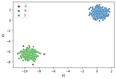
display_categories(dbscan,two_blobs_outliers)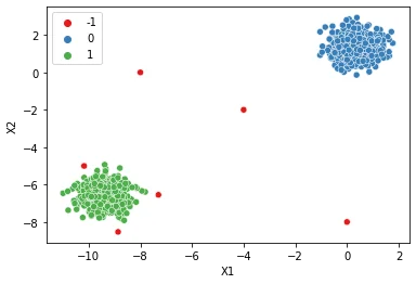
Epsilon
eps : float, default=0.5
| The maximum distance between two samples for one to be considered |
|---|
| as in the neighborhood of the other. This is not a maximum bound |
| on the distances of points within a cluster. This is the most |
| important DBSCAN parameter to choose appropriately for your data set |
| and distance function. |
# Tiny Epsilon --> Tiny Max Distance --> Everything is an outlier (class=-1)
dbscan = DBSCAN(eps=0.001)
display_categories(dbscan,two_blobs_outliers)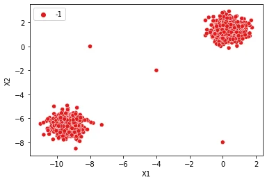
# Huge Epsilon --> Huge Max Distance --> Everything is in the same cluster (class=0)
dbscan = DBSCAN(eps=10)
display_categories(dbscan,two_blobs_outliers)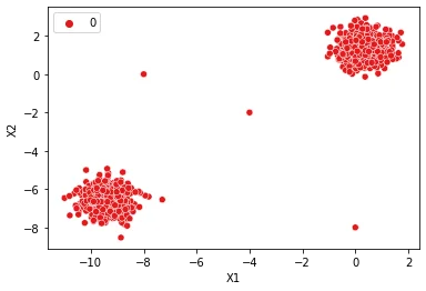
# How to find a good epsilon?
plt.figure(figsize=(10,6),dpi=200)
dbscan = DBSCAN(eps=1)
display_categories(dbscan,two_blobs_outliers)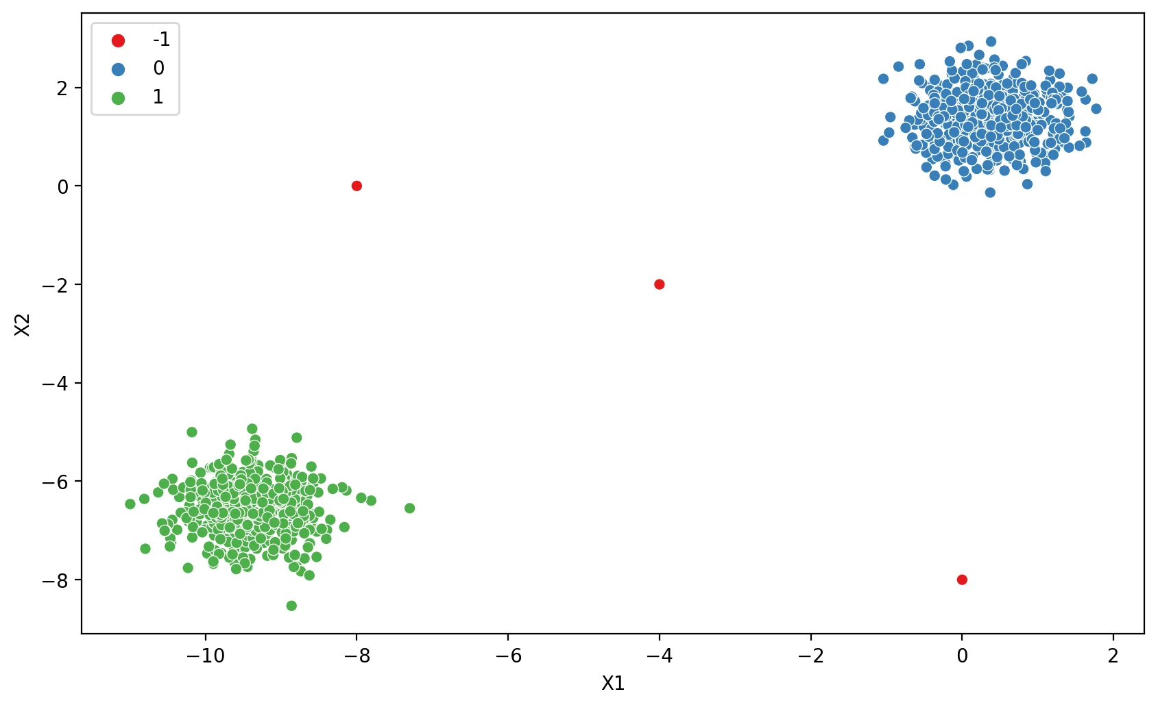
dbscan.labels_array([ 0, 1, 0, ..., -1, -1, -1], dtype=int64)dbscan.labels_ == -1array([False, False, False, ..., True, True, True])np.sum(dbscan.labels_ == -1)3100 * np.sum(dbscan.labels_ == -1) / len(dbscan.labels_)0.29910269192422734Charting reasonable Epsilon values
# bend the knee! https://raghavan.usc.edu/papers/kneedle-simplex11.pdf# np.arange(start=0.01,stop=10,step=0.01)outlier_percent = []
number_of_outliers = []
for eps in np.linspace(0.001,10,100):
# Create Model
dbscan = DBSCAN(eps=eps)
dbscan.fit(two_blobs_outliers)
# Log Number of Outliers
number_of_outliers.append(np.sum(dbscan.labels_ == -1))
# Log percentage of points that are outliers
perc_outliers = 100 * np.sum(dbscan.labels_ == -1) / len(dbscan.labels_)
outlier_percent.append(perc_outliers)sns.lineplot(x=np.linspace(0.001,10,100),y=outlier_percent)
plt.ylabel("Percentage of Points Classified as Outliers")
plt.xlabel("Epsilon Value")Text(0.5, 0, 'Epsilon Value')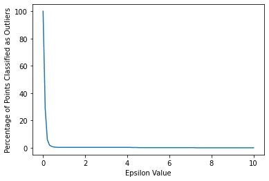
sns.lineplot(x=np.linspace(0.001,10,100),y=number_of_outliers)
plt.ylabel("Number of Points Classified as Outliers")
plt.xlabel("Epsilon Value")
plt.xlim(0,1)(0.0, 1.0)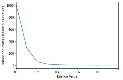
Do we want to think in terms of percentage targeting instead?
If so, you could "target" a percentage, like choose a range producing 1%-5% as outliers.
sns.lineplot(x=np.linspace(0.001,10,100),y=outlier_percent)
plt.ylabel("Percentage of Points Classified as Outliers")
plt.xlabel("Epsilon Value")
plt.ylim(0,5)
plt.xlim(0,2)
plt.hlines(y=1,xmin=0,xmax=2,colors='red',ls='--')<matplotlib.collections.LineCollection at 0x19a401a0af0>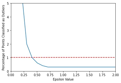
# How to find a good epsilon?
dbscan = DBSCAN(eps=0.4)
display_categories(dbscan,two_blobs_outliers)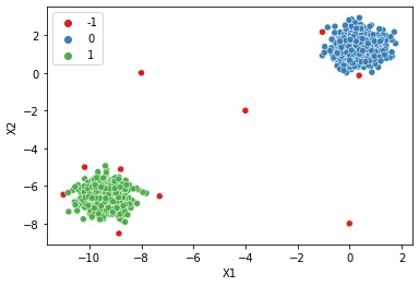
Do we want to think in terms of number of outliers targeting instead?
If so, you could "target" a number of outliers, such as 3 points as outliers.
sns.lineplot(x=np.linspace(0.001,10,100),y=number_of_outliers)
plt.ylabel("Number of Points Classified as Outliers")
plt.xlabel("Epsilon Value")
plt.ylim(0,10)
plt.xlim(0,6)
plt.hlines(y=3,xmin=0,xmax=10,colors='red',ls='--')<matplotlib.collections.LineCollection at 0x19a40070670>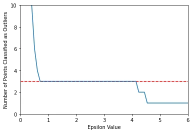
# How to find a good epsilon?
dbscan = DBSCAN(eps=0.75)
display_categories(dbscan,two_blobs_outliers)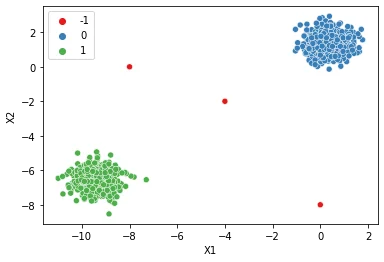
Minimum Samples
| min_samples : int, default=5 |
|---|
| The number of samples (or total weight) in a neighborhood for a point |
| to be considered as a core point. This includes the point itself. |
How to choose minimum number of points?
https://stats.stackexchange.com/questions/88872/a-routine-to-choose-eps-and-minpts-for-dbscan
outlier_percent = []

for n in np.arange(1,100):

    # Create Model
    dbscan = DBSCAN(min_samples=n)
    dbscan.fit(two_blobs_outliers)

    # Log percentage of points that are outliers
    perc_outliers = 100 * np.sum(dbscan.labels_ == -1) / len(dbscan.labels_)

outlier_percent.append(perc_outliers)sns.lineplot(x=np.arange(1,100),y=outlier_percent)
plt.ylabel("Percentage of Points Classified as Outliers")
plt.xlabel("Minimum Number of Samples")Text(0.5, 0, 'Minimum Number of Samples')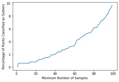
num_dim = two_blobs_outliers.shape[1]

dbscan = DBSCAN(min_samples=2*num_dim)
display_categories(dbscan,two_blobs_outliers)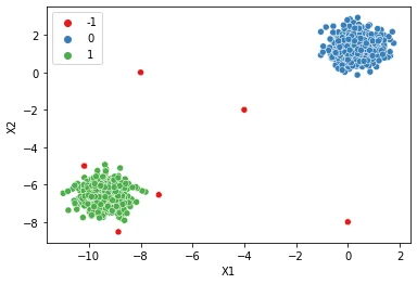
num_dim = two_blobs_outliers.shape[1]

dbscan = DBSCAN(eps=0.75,min_samples=2*num_dim)
display_categories(dbscan,two_blobs_outliers)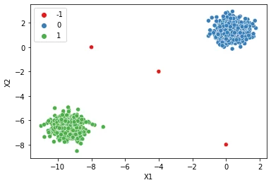
dbscan = DBSCAN(min_samples=1)
display_categories(dbscan,two_blobs_outliers)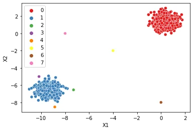
dbscan = DBSCAN(eps=0.75,min_samples=1)
display_categories(dbscan,two_blobs_outliers)