Dealing with Outliers
In statistics, an outlier is a data point that differs significantly from other observations.An outlier may be due to variability in the measurement or it may indicate experimental error; the latter are sometimes excluded from the data set. An outlier can cause serious problems in statistical analyses.
Remember that even if a data point is an outlier, its still a data point! Carefully consider your data, its sources, and your goals whenver deciding to remove an outlier. Each case is different!
Lecture Goals
- Understand different mathmatical definitions of outliers
- Use Python tools to recognize outliers and remove them
Useful Links
Imports
Generating Data
# Choose a mean,standard deviation, and number of samples

def create_ages(mu=50,sigma=13,num_samples=100,seed=42):

    # Set a random seed in the same cell as the random call to get the same values as us
    # We set seed to 42 (42 is an arbitrary choice from Hitchhiker's Guide to the Galaxy)
    np.random.seed(seed)

    sample_ages = np.random.normal(loc=mu,scale=sigma,size=num_samples)
    sample_ages = np.round(sample_ages,decimals=0)

return sample_agessample = create_ages()samplearray([56., 48., 58., 70., 47., 47., 71., 60., 44., 57., 44., 44., 53.,
25., 28., 43., 37., 54., 38., 32., 69., 47., 51., 31., 43., 51.,
35., 55., 42., 46., 42., 74., 50., 36., 61., 34., 53., 25., 33.,
53., 60., 52., 48., 46., 31., 41., 44., 64., 54., 27., 54., 45.,
41., 58., 63., 62., 39., 46., 54., 63., 44., 48., 36., 34., 61.,3 more lines
       68., 49., 63., 55., 42., 55., 70., 50., 70., 16., 61., 51., 46.,
       51., 24., 47., 55., 69., 43., 39., 43., 62., 54., 43., 57., 51.,
       63., 41., 46., 45., 31., 54., 53., 50., 47.])
Visualize and Describe the Data
sns.distplot(sample,bins=10,kde=False)<AxesSubplot:>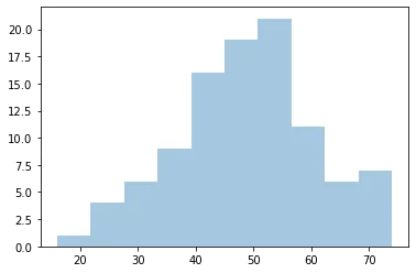
sns.boxplot(sample)<AxesSubplot:>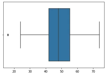
ser = pd.Series(sample)
ser.describe()count 100.00000
mean 48.66000
std 11.82039
min 16.00000
25% 42.000004 more lines
50%       48.00000
75%       55.25000
max       74.00000
dtype: float64
Trimming or Fixing Based Off Domain Knowledge
If we know we're dealing with a dataset pertaining to voting age (18 years old in the USA), then it makes sense to either drop anything less than that OR fix values lower than 18 and push them up to 18.
ser[ser > 18]0 56.0
1 48.0
2 58.0
3 70.0
4 47.07 more lines
      ...
95    31.0
96    54.0
97    53.0
98    50.0
99    47.0
Length: 99, dtype: float64# It dropped one person
len(ser[ser > 18])99def fix_values(age):
if age < 18:
return 18
else:
return age# "Fixes" one person's age
ser.apply(fix_values)0 56.0
1 48.0
2 58.0
3 70.0
4 47.07 more lines
      ...
95    31.0
96    54.0
97    53.0
98    50.0
99    47.0
Length: 100, dtype: float64len(ser.apply(fix_values))100There are many ways to identify and remove outliers:
- Trimming based off a provided value
- Capping based off IQR or STD
- https://towardsdatascience.com/ways-to-detect-and-remove-the-outliers-404d16608dba
- https://towardsdatascience.com/5-ways-to-detect-outliers-that-every-data-scientist-should-know-python-code-70a54335a623
Ames Data Set
Let's explore any extreme outliers in our Ames Housing Data Set
df = pd.read_csv("../DATA/Ames_Housing_Data.csv")df.head()PID
MS SubClass
MS Zoning
Lot Frontage
Lot Area127 more lines
Street
Alley
Lot Shape
Land Contour
Utilities
...
Pool Area
Pool QC
Fence
Misc Feature
Misc Val
Mo Sold
Yr Sold
Sale Type
Sale Condition
SalePrice
0
526301100
20
RL
141.0
31770
Pave
NaN
IR1
Lvl
AllPub
...
0
NaN
NaN
NaN
0
5
2010
WD
Normal
215000
1
526350040
20
RH
80.0
11622
Pave
NaN
Reg
Lvl
AllPub
...
0
NaN
MnPrv
NaN
0
6
2010
WD
Normal
105000
2
526351010
20
RL
81.0
14267
Pave
NaN
IR1
Lvl
AllPub
...
0
NaN
NaN
Gar2
12500
6
2010
WD
Normal
172000
3
526353030
20
RL
93.0
11160
Pave
NaN
Reg
Lvl
AllPub
...
0
NaN
NaN
NaN
0
4
2010
WD
Normal
244000
4
527105010
60
RL
74.0
13830
Pave
NaN
IR1
Lvl
AllPub
...
0
NaN
MnPrv
NaN
0
3
2010
WD
Normal
189900
5 rows × 81 columnssns.heatmap(df.corr())<AxesSubplot:>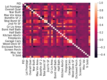
df.corr()['SalePrice'].sort_values()PID -0.246521
Enclosed Porch -0.128787
Kitchen AbvGr -0.119814
Overall Cond -0.101697
MS SubClass -0.08509234 more lines
Low Qual Fin SF   -0.037660
Bsmt Half Bath    -0.035835
Yr Sold           -0.030569
Misc Val          -0.015691
BsmtFin SF 2       0.005891
3Ssn Porch         0.032225
Mo Sold            0.035259
Pool Area          0.068403
Screen Porch       0.112151
Bedroom AbvGr      0.143913
Bsmt Unf SF        0.182855
Lot Area           0.266549
2nd Flr SF         0.269373
Bsmt Full Bath     0.276050
Half Bath          0.285056
Open Porch SF      0.312951
Wood Deck SF       0.327143
Lot Frontage       0.357318
BsmtFin SF 1       0.432914
Fireplaces         0.474558
TotRms AbvGrd      0.495474
Mas Vnr Area       0.508285
Garage Yr Blt      0.526965
Year Remod/Add     0.532974
Full Bath          0.545604
Year Built         0.558426
1st Flr SF         0.621676
Total Bsmt SF      0.632280
Garage Area        0.640401
Garage Cars        0.647877
Gr Liv Area        0.706780
Overall Qual       0.799262
SalePrice          1.000000
Name: SalePrice, dtype: float64sns.distplot(df["SalePrice"])<AxesSubplot:xlabel='SalePrice'>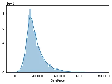
sns.scatterplot(x='Overall Qual',y='SalePrice',data=df)<AxesSubplot:xlabel='Overall Qual', ylabel='SalePrice'>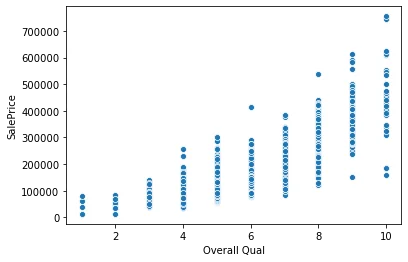
df[(df['Overall Qual']>8) & (df['SalePrice']<200000)]PID
MS SubClass
MS Zoning
Lot Frontage
Lot Area105 more lines
Street
Alley
Lot Shape
Land Contour
Utilities
...
Pool Area
Pool QC
Fence
Misc Feature
Misc Val
Mo Sold
Yr Sold
Sale Type
Sale Condition
SalePrice
1182
533350090
60
RL
NaN
24572
Pave
NaN
IR1
Lvl
AllPub
...
0
NaN
NaN
NaN
0
6
2008
WD
Family
150000
1498
908154235
60
RL
313.0
63887
Pave
NaN
IR3
Bnk
AllPub
...
480
Gd
NaN
NaN
0
1
2008
New
Partial
160000
2180
908154195
20
RL
128.0
39290
Pave
NaN
IR1
Bnk
AllPub
...
0
NaN
NaN
Elev
17000
10
2007
New
Partial
183850
2181
908154205
60
RL
130.0
40094
Pave
NaN
IR1
Bnk
AllPub
...
0
NaN
NaN
NaN
0
10
2007
New
Partial
184750
4 rows × 81 columnssns.scatterplot(x='Gr Liv Area',y='SalePrice',data=df)<AxesSubplot:xlabel='Gr Liv Area', ylabel='SalePrice'>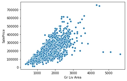
df[(df['Gr Liv Area']>4000) & (df['SalePrice']<400000)]PID
MS SubClass
MS Zoning
Lot Frontage
Lot Area83 more lines
Street
Alley
Lot Shape
Land Contour
Utilities
...
Pool Area
Pool QC
Fence
Misc Feature
Misc Val
Mo Sold
Yr Sold
Sale Type
Sale Condition
SalePrice
1498
908154235
60
RL
313.0
63887
Pave
NaN
IR3
Bnk
AllPub
...
480
Gd
NaN
NaN
0
1
2008
New
Partial
160000
2180
908154195
20
RL
128.0
39290
Pave
NaN
IR1
Bnk
AllPub
...
0
NaN
NaN
Elev
17000
10
2007
New
Partial
183850
2181
908154205
60
RL
130.0
40094
Pave
NaN
IR1
Bnk
AllPub
...
0
NaN
NaN
NaN
0
10
2007
New
Partial
184750
3 rows × 81 columnsdf[(df['Gr Liv Area']>4000) & (df['SalePrice']<400000)].indexInt64Index([1498, 2180, 2181], dtype='int64')ind_drop = df[(df['Gr Liv Area']>4000) & (df['SalePrice']<400000)].indexdf = df.drop(ind_drop,axis=0)sns.scatterplot(x='Gr Liv Area',y='SalePrice',data=df)<AxesSubplot:xlabel='Gr Liv Area', ylabel='SalePrice'>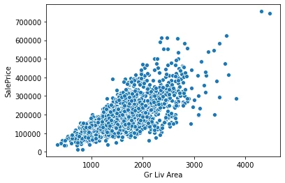
sns.scatterplot(x='Overall Qual',y='SalePrice',data=df)<AxesSubplot:xlabel='Overall Qual', ylabel='SalePrice'>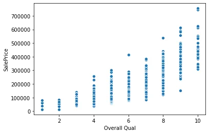
df.to_csv("../DATA/Ames_outliers_removed.csv",index=False)