Supervised Learning Capstone Project - Tree Methods Focus - SOLUTIONS
Make sure to review the introduction video to understand the 3 ways of approaching this project exercise!
Ways to approach the project:
- Open a new notebook, read in the data, and then analyze and visualize whatever you want, then create a predictive model.
- Use this notebook as a general guide, completing the tasks in bold shown below.
- Skip to the solutions notebook and video, and treat project at a more relaxing code along walkthrough lecture series.
GOAL: Create a model to predict whether or not a customer will Churn .
Complete the Tasks in Bold Below!
Part 0: Imports and Read in the Data
TASK: Run the filled out cells below to import libraries and read in your data. The data file is "Telco-Customer-Churn.csv"
# RUN THESE CELLS TO START THE PROJECT!
import numpy as np
import pandas as pd
import matplotlib.pyplot as plt
import seaborn as snsdf = pd.read_csv('../DATA/Telco-Customer-Churn.csv')df.head()customerID
gender
SeniorCitizen
Partner
Dependents127 more lines
tenure
PhoneService
MultipleLines
InternetService
OnlineSecurity
...
DeviceProtection
TechSupport
StreamingTV
StreamingMovies
Contract
PaperlessBilling
PaymentMethod
MonthlyCharges
TotalCharges
Churn
0
7590-VHVEG
Female
0
Yes
No
1
No
No phone service
DSL
No
...
No
No
No
No
Month-to-month
Yes
Electronic check
29.85
29.85
No
1
5575-GNVDE
Male
0
No
No
34
Yes
No
DSL
Yes
...
Yes
No
No
No
One year
No
Mailed check
56.95
1889.50
No
2
3668-QPYBK
Male
0
No
No
2
Yes
No
DSL
Yes
...
No
No
No
No
Month-to-month
Yes
Mailed check
53.85
108.15
Yes
3
7795-CFOCW
Male
0
No
No
45
No
No phone service
DSL
Yes
...
Yes
Yes
No
No
One year
No
Bank transfer (automatic)
42.30
1840.75
No
4
9237-HQITU
Female
0
No
No
2
Yes
No
Fiber optic
No
...
No
No
No
No
Month-to-month
Yes
Electronic check
70.70
151.65
Yes
5 rows × 21 columns
Part 1: Quick Data Check
TASK: Confirm quickly with .info() methods the datatypes and non-null values in your dataframe.
# CODE HEREdf.info()<class 'pandas.core.frame.DataFrame'>
RangeIndex: 7032 entries, 0 to 7031
Data columns (total 21 columns):
# Column Non-Null Count Dtype
--- ------ -------------- ----- 23 more lines
 0   customerID        7032 non-null   object
 1   gender            7032 non-null   object
 2   SeniorCitizen     7032 non-null   int64
 3   Partner           7032 non-null   object
 4   Dependents        7032 non-null   object
 5   tenure            7032 non-null   int64
 6   PhoneService      7032 non-null   object
 7   MultipleLines     7032 non-null   object
 8   InternetService   7032 non-null   object
 9   OnlineSecurity    7032 non-null   object
 10  OnlineBackup      7032 non-null   object
 11  DeviceProtection  7032 non-null   object
 12  TechSupport       7032 non-null   object
 13  StreamingTV       7032 non-null   object
 14  StreamingMovies   7032 non-null   object
 15  Contract          7032 non-null   object
 16  PaperlessBilling  7032 non-null   object
 17  PaymentMethod     7032 non-null   object
 18  MonthlyCharges    7032 non-null   float64
 19  TotalCharges      7032 non-null   float64
 20  Churn             7032 non-null   object
dtypes: float64(2), int64(2), object(17)
memory usage: 1.1+ MB
TASK: Get a quick statistical summary of the numeric columns with .describe() , you should notice that many columns are categorical, meaning you will eventually need to convert them to dummy variables.
# CODE HEREdf.describe()SeniorCitizen
tenure
MonthlyCharges
TotalCharges
count39 more lines
7032.000000
7032.000000
7032.000000
7032.000000
mean
0.162400
32.421786
64.798208
2283.300441
std
0.368844
24.545260
30.085974
2266.771362
min
0.000000
1.000000
18.250000
18.800000
25%
0.000000
9.000000
35.587500
401.450000
50%
0.000000
29.000000
70.350000
1397.475000
75%
0.000000
55.000000
89.862500
3794.737500
max
1.000000
72.000000
118.750000
8684.800000
Part 2: Exploratory Data Analysis
General Feature Exploration
TASK: Confirm that there are no NaN cells by displaying NaN values per feature column.
# CODE HEREdf.isna().sum()customerID 0
gender 0
SeniorCitizen 0
Partner 0
Dependents 017 more lines
tenure              0
PhoneService        0
MultipleLines       0
InternetService     0
OnlineSecurity      0
OnlineBackup        0
DeviceProtection    0
TechSupport         0
StreamingTV         0
StreamingMovies     0
Contract            0
PaperlessBilling    0
PaymentMethod       0
MonthlyCharges      0
TotalCharges        0
Churn               0
dtype: int64
TASK:Display the balance of the class labels (Churn) with a Count Plot.
# CODE HEREsns.countplot(data=df,x='Churn')<AxesSubplot:xlabel='Churn', ylabel='count'>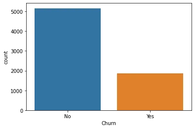
TASK: Explore the distrbution of TotalCharges between Churn categories with a Box Plot or Violin Plot.
# CODE HEREsns.violinplot(data=df,x='Churn',y='TotalCharges')<AxesSubplot:xlabel='Churn', ylabel='TotalCharges'>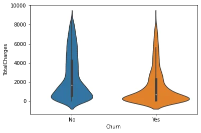
TASK: Create a boxplot showing the distribution of TotalCharges per Contract type, also add in a hue coloring based on the Churn class.
#CODE HEREplt.figure(figsize=(10,4),dpi=200)
sns.boxplot(data=df,y='TotalCharges',x='Contract',hue='Churn')
plt.legend(loc=(1.1,0.5))<matplotlib.legend.Legend at 0x2d1eb25c100>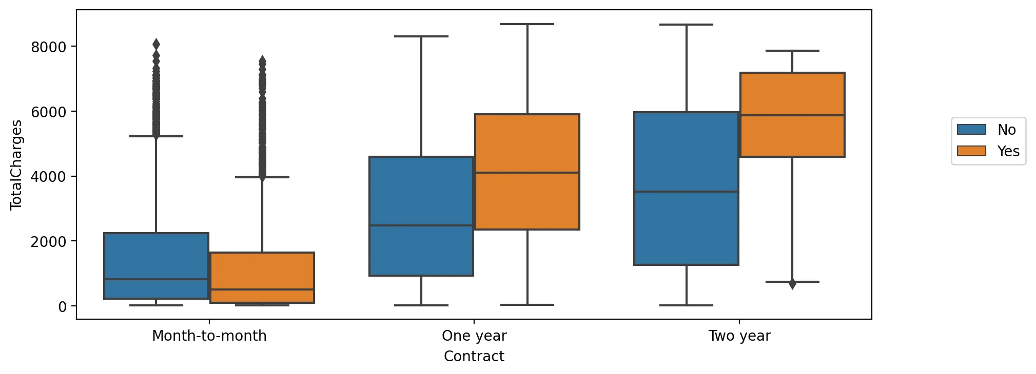
TASK: Create a bar plot showing the correlation of the following features to the class label. Keep in mind, for the categorical features, you will need to convert them into dummy variables first, as you can only calculate correlation for numeric features.
['gender', 'SeniorCitizen', 'Partner', 'Dependents','PhoneService', 'MultipleLines', 'OnlineSecurity', 'OnlineBackup', 'DeviceProtection', 'TechSupport', 'InternetService', 'StreamingTV', 'StreamingMovies', 'Contract', 'PaperlessBilling', 'PaymentMethod']
*Note, we specifically listed only the features above, you should not check the correlation for every feature, as some features have too many unique instances for such an analysis, such as customerID*
#CODE HEREdf.columnsIndex(['customerID', 'gender', 'SeniorCitizen', 'Partner', 'Dependents',
'tenure', 'PhoneService', 'MultipleLines', 'InternetService',
'OnlineSecurity', 'OnlineBackup', 'DeviceProtection', 'TechSupport',
'StreamingTV', 'StreamingMovies', 'Contract', 'PaperlessBilling',
'PaymentMethod', 'MonthlyCharges', 'TotalCharges', 'Churn'],1 more line
dtype='object')corr_df = pd.get_dummies(df[['gender', 'SeniorCitizen', 'Partner', 'Dependents','PhoneService', 'MultipleLines', 'InternetService',
'OnlineSecurity', 'OnlineBackup', 'DeviceProtection', 'TechSupport','StreamingTV', 'StreamingMovies', 'Contract', 'PaperlessBilling',
'PaymentMethod','Churn']]).corr()corr_df['Churn_Yes'].sort_values().iloc[1:-1]Contract_Two year -0.301552
StreamingMovies_No internet service -0.227578
StreamingTV_No internet service -0.227578
TechSupport_No internet service -0.227578
DeviceProtection_No internet service -0.22757838 more lines
OnlineBackup_No internet service          -0.227578
OnlineSecurity_No internet service        -0.227578
InternetService_No                        -0.227578
PaperlessBilling_No                       -0.191454
Contract_One year                         -0.178225
OnlineSecurity_Yes                        -0.171270
TechSupport_Yes                           -0.164716
Dependents_Yes                            -0.163128
Partner_Yes                               -0.149982
PaymentMethod_Credit card (automatic)     -0.134687
InternetService_DSL                       -0.124141
PaymentMethod_Bank transfer (automatic)   -0.118136
PaymentMethod_Mailed check                -0.090773
OnlineBackup_Yes                          -0.082307
DeviceProtection_Yes                      -0.066193
MultipleLines_No                          -0.032654
MultipleLines_No phone service            -0.011691
PhoneService_No                           -0.011691
gender_Male                               -0.008545
gender_Female                              0.008545
PhoneService_Yes                           0.011691
MultipleLines_Yes                          0.040033
StreamingMovies_Yes                        0.060860
StreamingTV_Yes                            0.063254
StreamingTV_No                             0.128435
StreamingMovies_No                         0.130920
Partner_No                                 0.149982
SeniorCitizen                              0.150541
Dependents_No                              0.163128
PaperlessBilling_Yes                       0.191454
DeviceProtection_No                        0.252056
OnlineBackup_No                            0.267595
PaymentMethod_Electronic check             0.301455
InternetService_Fiber optic                0.307463
TechSupport_No                             0.336877
OnlineSecurity_No                          0.342235
Contract_Month-to-month                    0.404565
Name: Churn_Yes, dtype: float64plt.figure(figsize=(10,4),dpi=200)
sns.barplot(x=corr_df['Churn_Yes'].sort_values().iloc[1:-1].index,y=corr_df['Churn_Yes'].sort_values().iloc[1:-1].values)
plt.title("Feature Correlation to Yes Churn")
plt.xticks(rotation=90);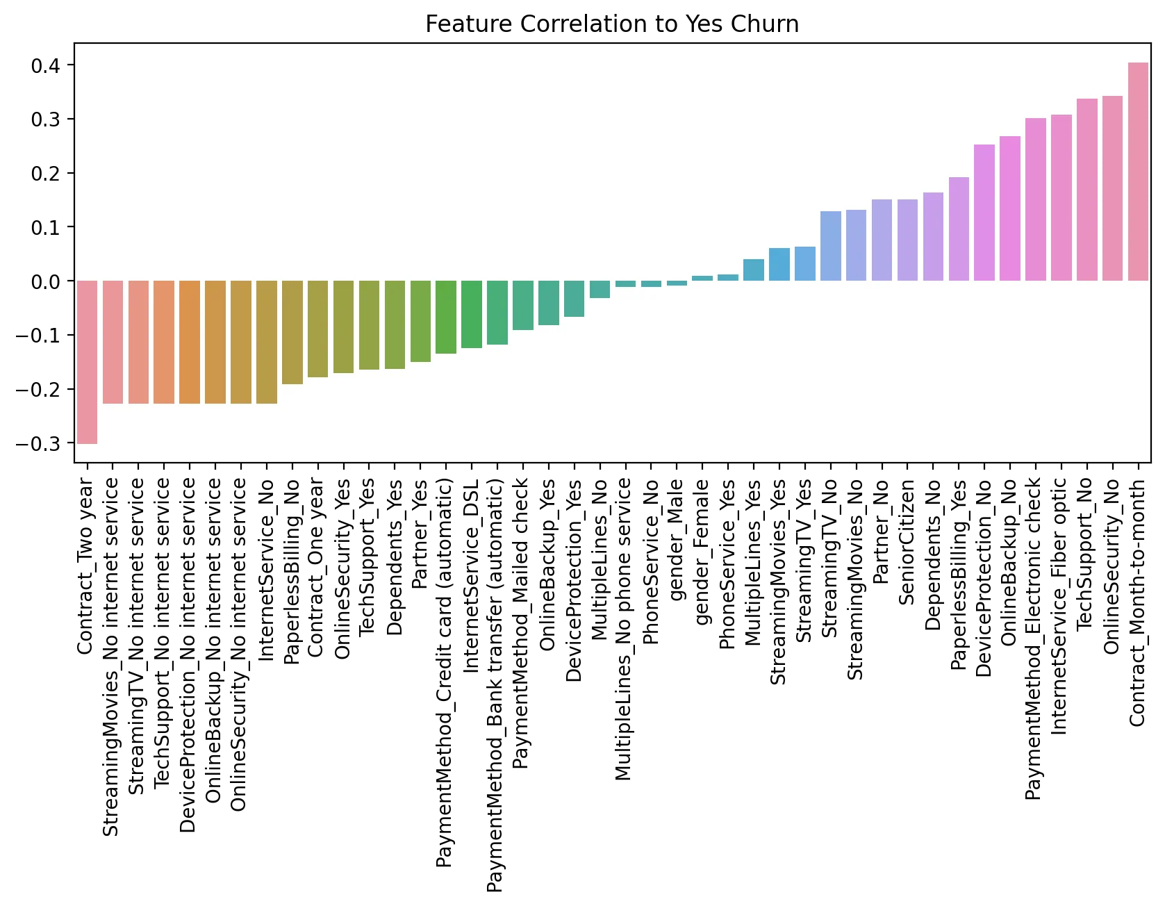
Part 3: Churn Analysis
This section focuses on segementing customers based on their tenure, creating "cohorts", allowing us to examine differences between customer cohort segments.
TASK: What are the 3 contract types available?
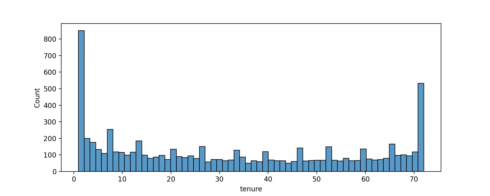
# CODE HEREdf['Contract'].unique()array(['Month-to-month', 'One year', 'Two year'], dtype=object)TASK: Create a histogram displaying the distribution of 'tenure' column, which is the amount of months a customer was or has been on a customer.
#CODE HEREplt.figure(figsize=(10,4),dpi=200)
sns.histplot(data=df,x='tenure',bins=60)<AxesSubplot:xlabel='tenure', ylabel='Count'>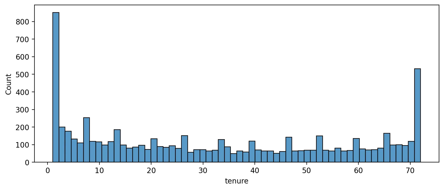
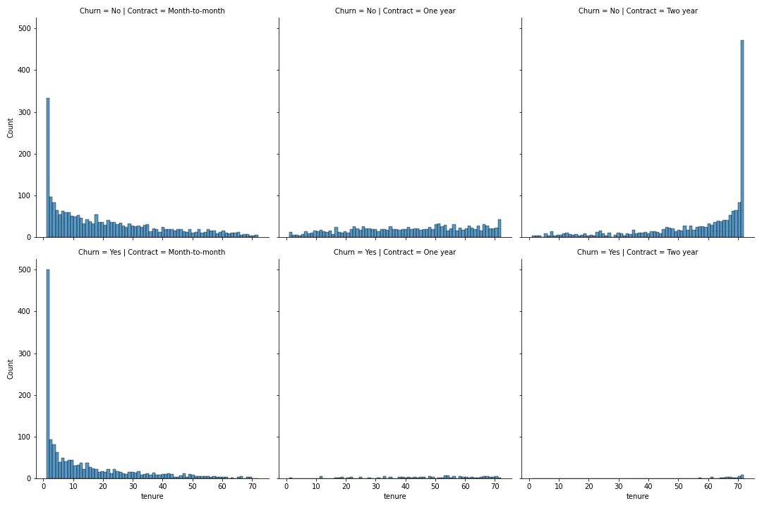
TASK: Now use the seaborn documentation as a guide to create histograms separated by two additional features, Churn and Contract.
#CODE HEREplt.figure(figsize=(10,3),dpi=200)
sns.displot(data=df,x='tenure',bins=70,col='Contract',row='Churn');<Figure size 2000x600 with 0 Axes>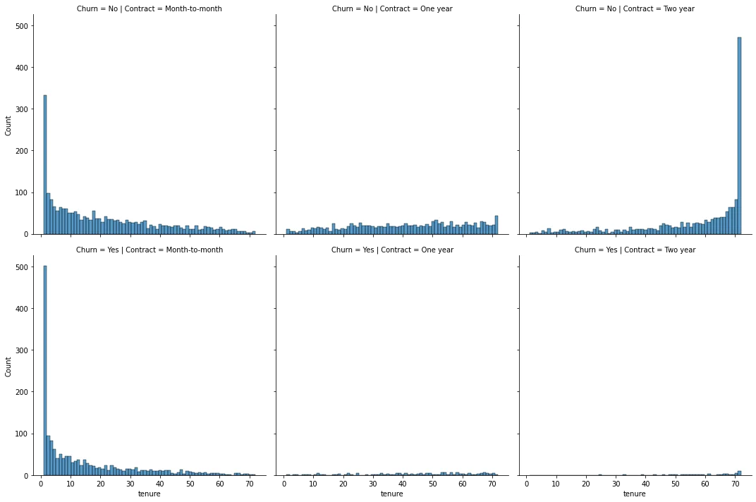
TASK: Display a scatter plot of Total Charges versus Monthly Charges, and color hue by Churn.
#CODE HEREdf.columnsIndex(['customerID', 'gender', 'SeniorCitizen', 'Partner', 'Dependents',
'tenure', 'PhoneService', 'MultipleLines', 'InternetService',
'OnlineSecurity', 'OnlineBackup', 'DeviceProtection', 'TechSupport',
'StreamingTV', 'StreamingMovies', 'Contract', 'PaperlessBilling',
'PaymentMethod', 'MonthlyCharges', 'TotalCharges', 'Churn'],1 more line
dtype='object')plt.figure(figsize=(10,4),dpi=200)
sns.scatterplot(data=df,x='MonthlyCharges',y='TotalCharges',hue='Churn', linewidth=0.5,alpha=0.5,palette='Dark2')<AxesSubplot:xlabel='MonthlyCharges', ylabel='TotalCharges'>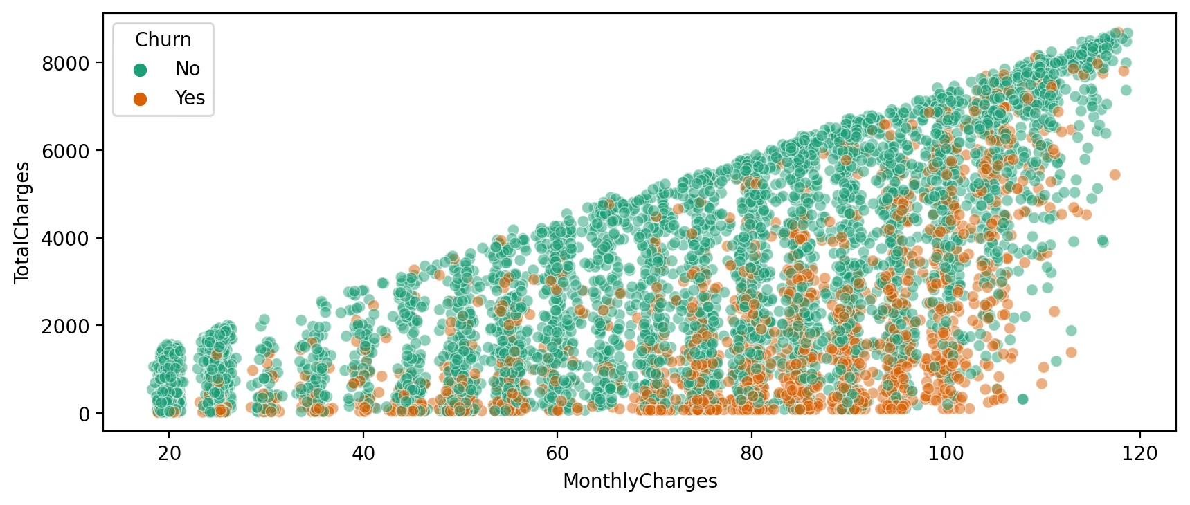
Creating Cohorts based on Tenure
Let's begin by treating each unique tenure length, 1 month, 2 month, 3 month...N months as its own cohort.
TASK: Treating each unique tenure group as a cohort, calculate the Churn rate (percentage that had Yes Churn) per cohort. For example, the cohort that has had a tenure of 1 month should have a Churn rate of 61.99%. You should have cohorts 1-72 months with a general trend of the longer the tenure of the cohort, the less of a churn rate. This makes sense as you are less likely to stop service the longer you've had it.
#CODE HEREno_churn = df.groupby(['Churn','tenure']).count().transpose()['No']
yes_churn = df.groupby(['Churn','tenure']).count().transpose()['Yes']churn_rate = 100 * yes_churn / (no_churn+yes_churn)churn_rate.transpose()['customerID']tenure
1 61.990212
2 51.680672
3 47.000000
4 47.1590918 more lines
5     48.120301
        ...
68     9.000000
69     8.421053
70     9.243697
71     3.529412
72     1.657459
Name: customerID, Length: 72, dtype: float64
TASK: Now that you have Churn Rate per tenure group 1-72 months, create a plot showing churn rate per months of tenure.
#CODE HEREplt.figure(figsize=(10,4),dpi=200)
churn_rate.iloc[0].plot()
plt.ylabel('Churn Percentage');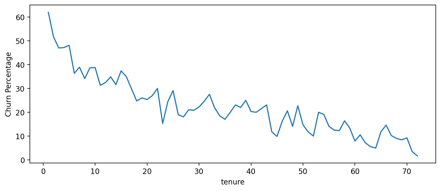
Broader Cohort Groups
TASK: Based on the tenure column values, create a new column called Tenure Cohort that creates 4 separate categories:
- '0-12 Months'
- '24-48 Months'
- '12-24 Months'
- 'Over 48 Months'
# CODE HEREdef cohort(tenure):
if tenure < 13:
return '0-12 Months'
elif tenure < 25:
return '12-24 Months'
elif tenure < 49:
return '24-48 Months'
else:
return "Over 48 Months"df['Tenure Cohort'] = df['tenure'].apply(cohort)df.head(10)[['tenure','Tenure Cohort']]tenure
Tenure Cohort
0
1
0-12 Months27 more lines
1
34
24-48 Months
2
2
0-12 Months
3
45
24-48 Months
4
2
0-12 Months
5
8
0-12 Months
6
22
12-24 Months
7
10
0-12 Months
8
28
24-48 Months
9
62
Over 48 Months
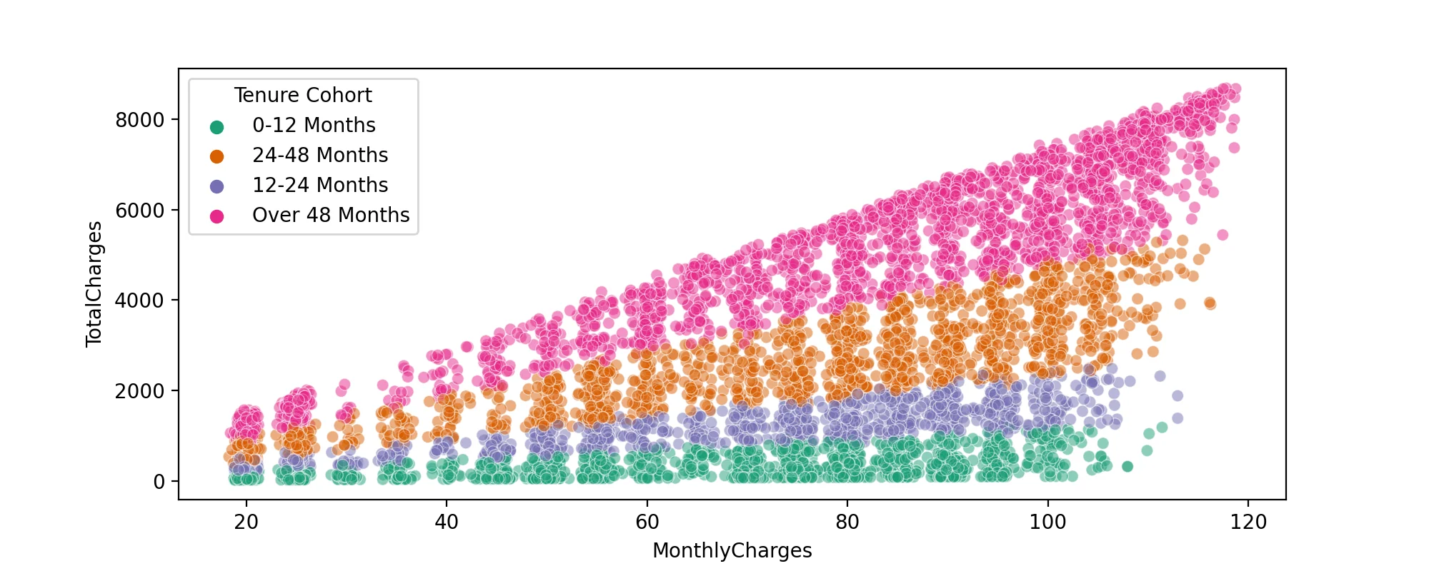
TASK: Create a scatterplot of Total Charges versus Monthly Charts,colored by Tenure Cohort defined in the previous task.
#CODE HEREplt.figure(figsize=(10,4),dpi=200)
sns.scatterplot(data=df,x='MonthlyCharges',y='TotalCharges',hue='Tenure Cohort', linewidth=0.5,alpha=0.5,palette='Dark2')<AxesSubplot:xlabel='MonthlyCharges', ylabel='TotalCharges'>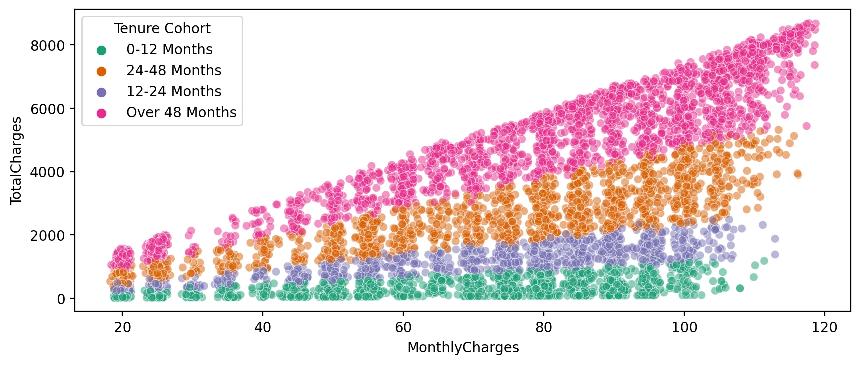
TASK: Create a count plot showing the churn count per cohort.
#CODE HEREplt.figure(figsize=(10,4),dpi=200)
sns.countplot(data=df,x='Tenure Cohort',hue='Churn')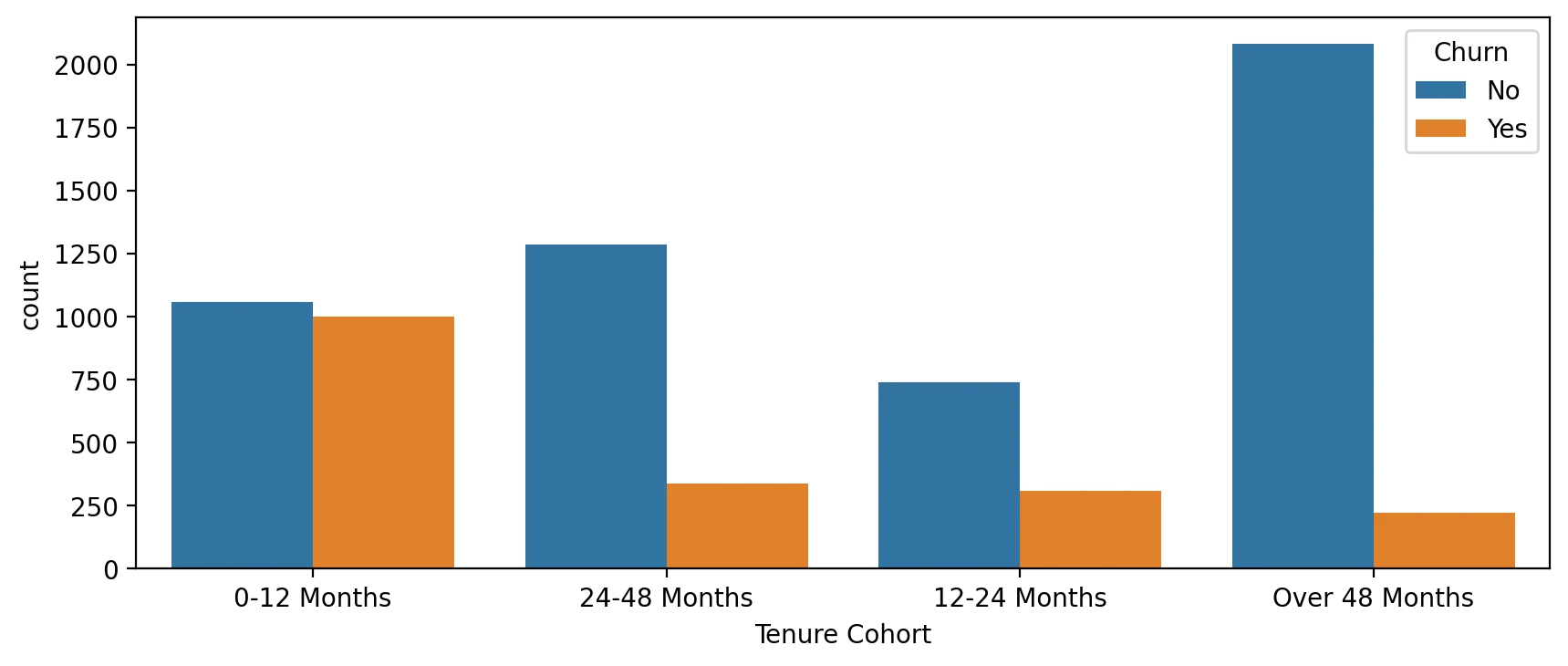
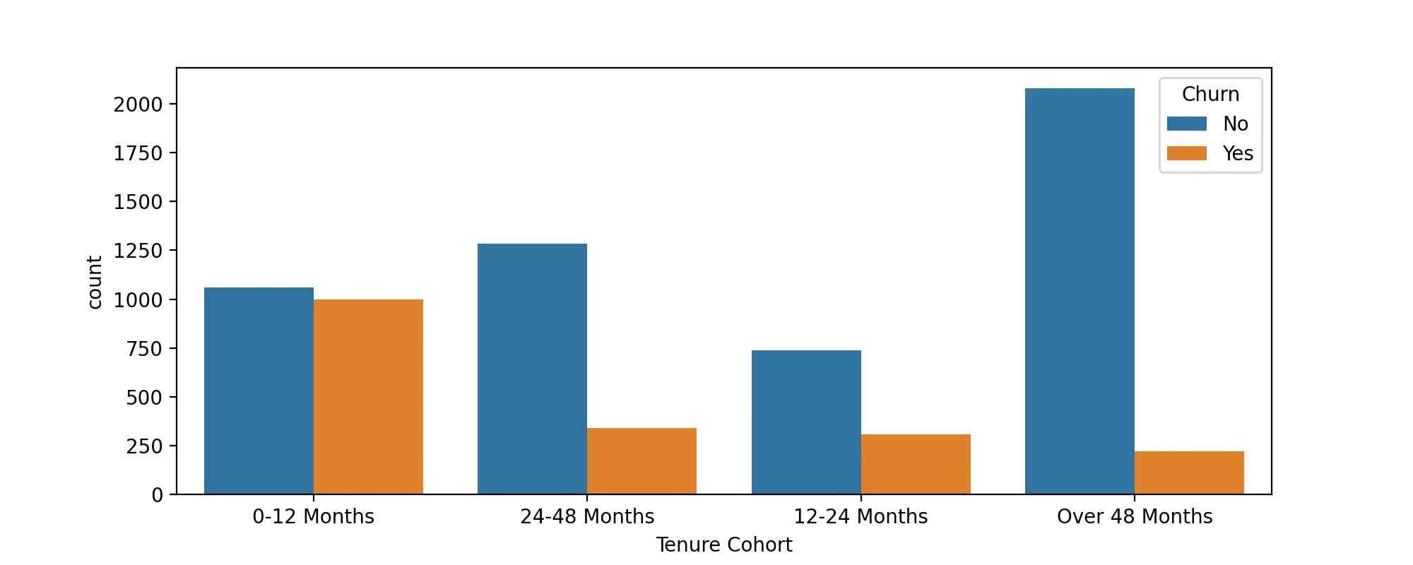
TASK: Create a grid of Count Plots showing counts per Tenure Cohort, separated out by contract type and colored by the Churn hue.
#CODE HEREplt.figure(figsize=(10,4),dpi=200)
sns.catplot(data=df,x='Tenure Cohort',hue='Churn',col='Contract',kind='count')<seaborn.axisgrid.FacetGrid at 0x2d1e3caafd0><Figure size 2000x800 with 0 Axes>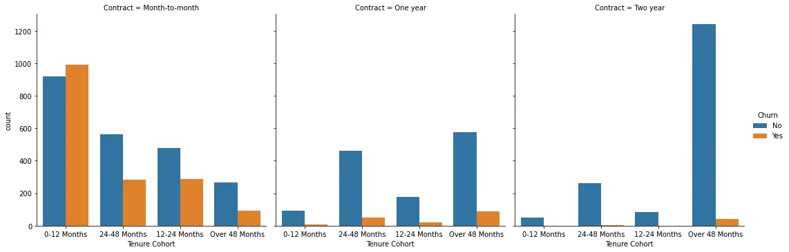
Part 4: Predictive Modeling
Let's explore 4 different tree based methods: A Single Decision Tree, Random Forest, AdaBoost, Gradient Boosting. Feel free to add any other supervised learning models to your comparisons!
Single Decision Tree
TASK : Separate out the data into X features and Y label. Create dummy variables where necessary and note which features are not useful and should be dropped.
#CODE HEREX = df.drop(['Churn','customerID'],axis=1)
X = pd.get_dummies(X,drop_first=True)y = df['Churn']TASK: Perform a train test split, holding out 10% of the data for testing. We'll use a random_state of 101 in the solutions notebook/video.
#CODE HEREfrom sklearn.model_selection import train_test_splitX_train, X_test, y_train, y_test = train_test_split(X, y, test_size=0.1, random_state=101)TASK: Decision Tree Perfomance. Complete the following tasks:
- Train a single decision tree model (feel free to grid search for optimal hyperparameters).
- Evaluate performance metrics from decision tree, including classification report and plotting a confusion matrix.
- Calculate feature importances from the decision tree.
- OPTIONAL: Plot your tree, note, the tree could be huge depending on your pruning, so it may crash your notebook if you display it with plot_tree.
from sklearn.tree import DecisionTreeClassifierdt = DecisionTreeClassifier(max_depth=6)dt.fit(X_train,y_train)DecisionTreeClassifier(max_depth=6)preds = dt.predict(X_test)from sklearn.metrics import accuracy_score,plot_confusion_matrix,classification_reportprint(classification_report(y_test,preds)) precision recall f1-score support
No 0.87 0.89 0.88 557
Yes 0.55 0.49 0.52 147
3 more lines
    accuracy                           0.81       704
   macro avg       0.71      0.69      0.70       704
weighted avg 0.80 0.81 0.81 704plot_confusion_matrix(dt,X_test,y_test)<sklearn.metrics._plot.confusion_matrix.ConfusionMatrixDisplay at 0x2d1e9601d90>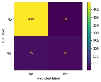
imp_feats = pd.DataFrame(data=dt.feature_importances_,index=X.columns,columns=['Feature Importance']).sort_values("Feature Importance")plt.figure(figsize=(14,6),dpi=200)
sns.barplot(data=imp_feats.sort_values('Feature Importance'),x=imp_feats.sort_values('Feature Importance').index,y='Feature Importance')
plt.xticks(rotation=90)
plt.title("Feature Importance for Decision Tree");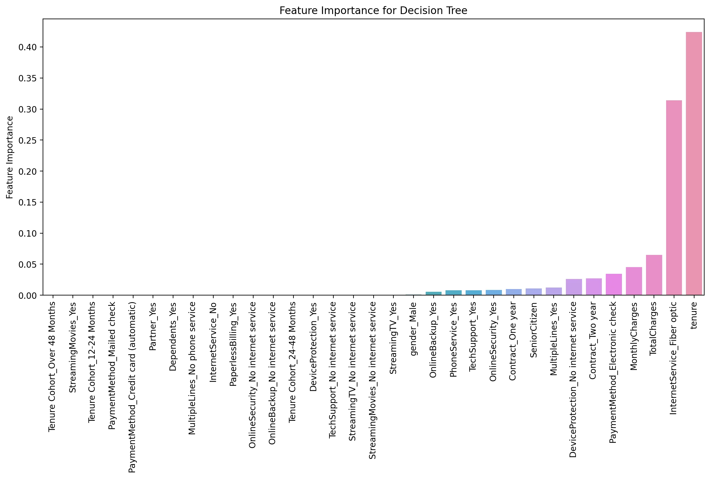
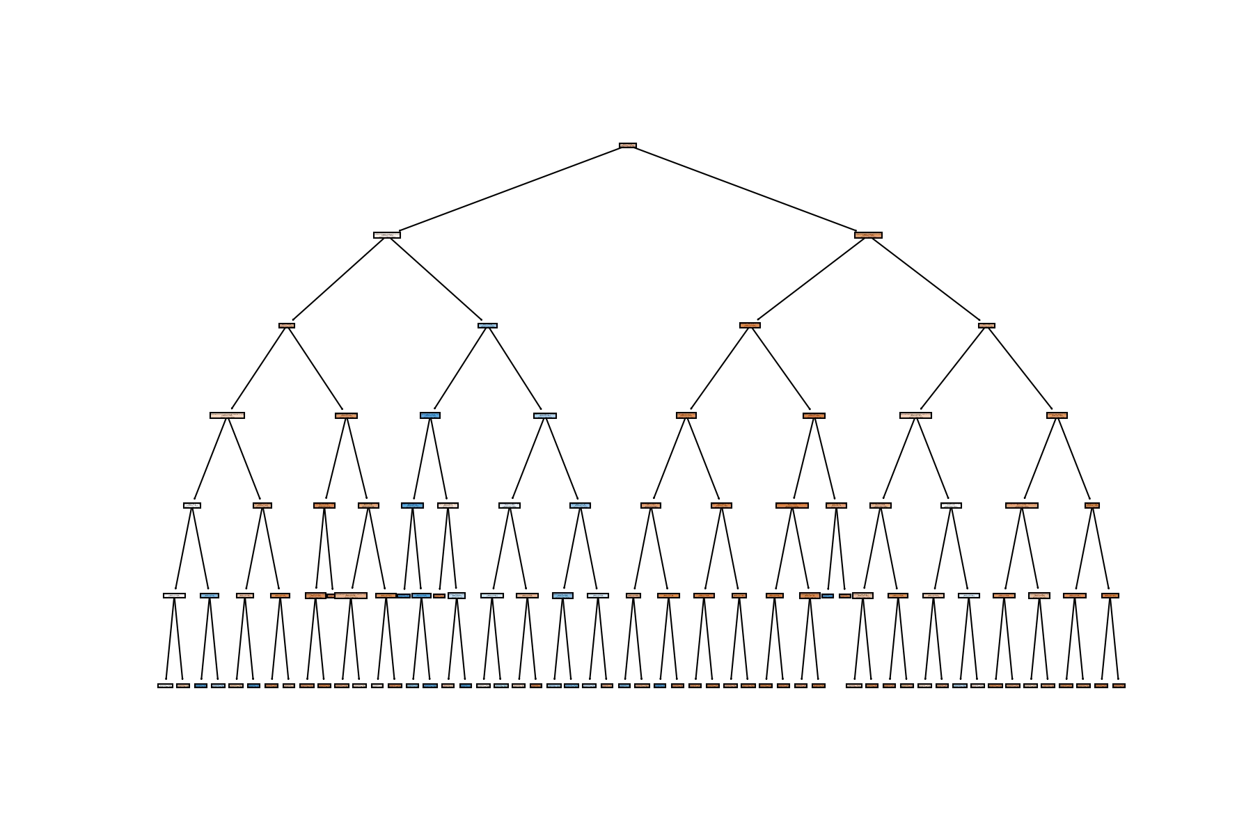
from sklearn.tree import plot_treeplt.figure(figsize=(12,8),dpi=150)
plot_tree(dt,filled=True,feature_names=X.columns);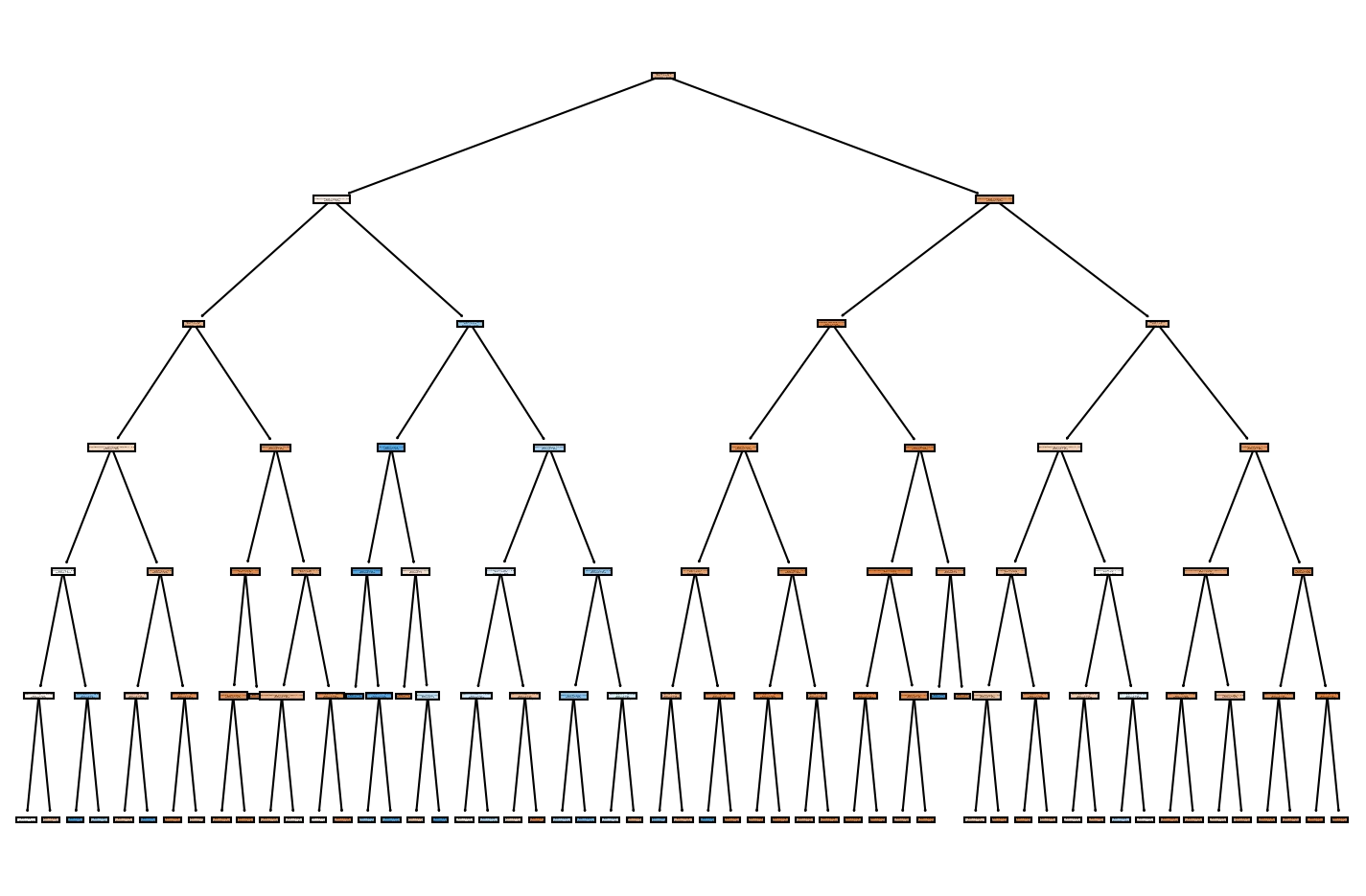
Random Forest
TASK: Create a Random Forest model and create a classification report and confusion matrix from its predicted results on the test set.
#CODE HEREfrom sklearn.ensemble import RandomForestClassifierrf = RandomForestClassifier(n_estimators=100)rf.fit(X_train,y_train)RandomForestClassifier()preds = rf.predict(X_test)print(classification_report(y_test,preds)) precision recall f1-score support
No 0.86 0.89 0.87 557
Yes 0.52 0.44 0.48 147
3 more lines
    accuracy                           0.80       704
   macro avg       0.69      0.67      0.68       704
weighted avg 0.79 0.80 0.79 704plot_confusion_matrix(dt,X_test,y_test)<sklearn.metrics._plot.confusion_matrix.ConfusionMatrixDisplay at 0x2d1e6a54040>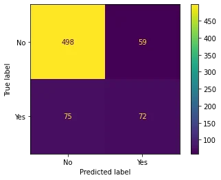
Boosted Trees
TASK: Use AdaBoost or Gradient Boosting to create a model and report back the classification report and plot a confusion matrix for its predicted results
#CODE HEREfrom sklearn.ensemble import GradientBoostingClassifier,AdaBoostClassifierada_model = AdaBoostClassifier()ada_model.fit(X_train,y_train)AdaBoostClassifier()preds = ada_model.predict(X_test)print(classification_report(y_test,preds)) precision recall f1-score support
No 0.88 0.90 0.89 557
Yes 0.60 0.54 0.57 147
3 more lines
    accuracy                           0.83       704
   macro avg       0.74      0.72      0.73       704
weighted avg 0.82 0.83 0.83 704plot_confusion_matrix(dt,X_test,y_test)<sklearn.metrics._plot.confusion_matrix.ConfusionMatrixDisplay at 0x2d1e9373a30>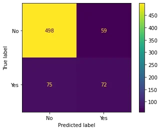
TASK: Analyze your results, which model performed best for you?
# With base models, we got best performance from an AdaBoostClassifier, but note, we didn't do any gridsearching AND most models performed about the same on the data set.